Method for Using Information Models and Queries to Connect HVAC Analytics and Data
Publication: Journal of Computing in Civil Engineering
Volume 37, Issue 6
Abstract
A significant portion of the energy used in building operations is wasted due to faults and poor operation. Despite volumes of research, the real-world use of analytics applications utilizing the data available from building systems is limited. Mapping the data points from building systems to analytics applications outside the building systems and automation requires expert labor, and is often done in point-to-point integrations. This study proposes a novel method for using queryable information models to connect data points of building systems to a centralized analytics platform without requiring a particular modeling technology. The method is explained in detail through a software architecture and is further demonstrated by walking through an implementation of an example rule from a rule-based fault detection method for air handling units. In the demonstration, an air handling unit is modeled with two different approaches, and the example analytic is connected to both. The method is shown to support reusing analytic implementations between building systems modeled with different approaches, with limited assumptions of the information models.
Introduction
In the operation of commercial buildings as much as 30% of HVAC and lighting system energy consumption is wasted due to poor operation and faults (Kim and Katipamula 2018). Buildings represent around 40% of the total energy consumption in the US and EU (Cao et al. 2016), making their energy waste reduction a significant global opportunity. One approach for optimizing energy consumption is the use of a monitoring-based commissioning (MBCx) process utilizing building analytics applications (Kramer et al. 2020). These applications analyze information gathered from the data points available in the building to inform the operators of aspects such as abnormal energy usage, poor control parameters, and suggested replacement schedule for equipment. For example, a study of the participants of the Smart Energy Analytics Campaign observed 7% median energy savings for users of Energy Management and Information Systems (EMIS) since installation, with the highest reported savings up to 28% and preliminary results suggesting the savings to be increasing over time (Kramer et al. 2020).
One acknowledged challenge to building analytics application setup is the lack of descriptions for building data points (Gunay et al. 2019). Various approaches to describing the data points exist, including the Haystack tagging framework (Project Haystack 2022) and semantic web ontologies such as Brick (Balaji et al. 2018) and RealEstateCore (Hammar et al. 2019). Further, American Society of Heating, Refrigerating and Air-Conditioning Engineers (ASHRAE)-sponsored development of the proposed Standard 223 (NIST 2021) seeks to unify efforts for semantic data models for buildings by leaning on earlier efforts. Although automated and semiautomated methods of classifying and creating other metadata for data points have been proposed (Wang et al. 2018), there are no one-size-fits-all solutions due to differences in the information requirements of analytics applications. Further, owners and operators of different buildings have different priorities and varying levels of willingness to invest in data descriptions and analytics.
Even with data point descriptions available, setting up and maintaining analytics applications requires mappings between data points and applicable analytics. Creating and maintaining these mappings is dependent on the work of building systems experts, making it expensive and thus contributing to the barrier of adoption (Harris et al. 2018). Applying analytics on a portfolio of buildings presents further challenges for data integration and management (Lin et al. 2022). Furthermore, more sophisticated analytics approaches require more investments and upkeep. For example, although the previously cited study of the participants of Smart Energy Analytics Campaign observed that users of more complicated fault detection and diagnostics (FDD) applications had greater energy savings compared with meter-level monitoring, it was also found that FDD implementations had a five times greater median base setup cost, with also greater recurring service costs and estimated in-house labor cost (Kramer et al. 2020).
To overcome some of the challenges related to creating and maintaining mappings between data points and applicable analytics in a centralized analytics platform, this study proposes a method for using information models and queries to bind time-series analytics to data points, such as sensors. Further, to support the data integration and management for a portfolio of buildings, the method does not require a particular information modeling technology or vocabulary. The proposed method is described as a software architecture with a narrow focus and in-depth explanations in contrast to more high-level architecture proposals (Pau et al. 2022; Marinakis 2020). An example prototype is built on semantic web technologies and knowledge-based fault detection rules.
The article is structured as follows. First, contemporary research related to connections of analytics applications and time-series data in the architecture, engineering, construction, and operations (AECO) field is reviewed. Next, the proposed method is described through a software architecture. Following that, an example application of air handling unit (AHU) fault detection is showcased. After that, the results and potential future research directions are discussed, before finally summarizing and concluding the work.
Related Work
Within the research body related to building analytics and MBCx for building systems, common subareas include the study of the methods themselves (how to utilize the data) and the study of data descriptions (how to annotate and classify the data). Other studies focus on high-level architectures where data integration is accounted for but not described in detail. The question of how to connect the various analytics methods with data annotated in different ways has received significantly less attention. This connection between time-series data and analysis engines is the focus of this study, and thus the existing research is reviewed through the question: how is the correct data provided to the analysis methods?
Existing analytics applications are commonly built around the assumption of a particular data model. For example, the MORTAR test bed (Fierro et al. 2019) was designed around Brick. Although several aspects of the architecture are independent of the data model, what MORTAR calls “portable applications” themselves contain the queries to find relevant data points, leading to a 1:1 relationship between queries and analytics or “portable applications.” On the other hand, the commercial SkySpark (SkyFoundry 2023) uses Project Haystack and is highly involved in its development.
Five general approaches to connecting data points to analytics were identified in previous literature:
•
point-to-point integration,
•
naming conventions,
•
data warehousing,
•
time-series in knowledge graphs, and
•
ontology-based data access (OBDA).
The remainder of this section discusses further definitions and examples of the different approaches.
Point-to-point integration requires some manual definition for each output. For example, OpenBAN sensor analytics middleware (Arjunan et al. 2015) uses so-called contextlets defined by users to connect sensor data streams to feature extraction methods and analytical algorithms. Sensor data streams are provided by input data adapters retrieving data from supported sources in a common format.
The greatest benefit of point-to-point integrations is simplicity, but this comes at the cost of scalability: adding new inputs (systems to analyze) and new outputs (desired analytics) leads to combinatorial explosion in the required number of integrations. Adding some logic or automation to define these integrations will then require the use of other integration methods, such as those described in the rest of this section.
Naming conventions rely on the use of a naming schema for data points and/or the things they relate to. The scope and information contents of naming conventions vary, but examples of information encoded in a name include the quantity observed by a data point, and the component or space the data point relates to. In one example, a taxonomical naming convention was developed to link data points to building information modeling (BIM) elements in Revit (Quinn et al. 2020). Another approach used a naming template for AHU data points to support FDD (Bruton et al. 2014).
Benefits of naming conventions include their relative simplicity (Quinn et al. 2020) and the fact that experts familiar with the schema can reason about the information encoded in the names. On the other hand, a drawback of naming conventions is that expanding their application is challenging, such as expanding the naming schema targeting AHUs (Bruton et al. 2014) to support FDD on a larger subset of the HVAC system. Further, some information, such as the relations of the spaces or components, is often hidden in implicit assumptions behind the naming convention.
Data warehousing is closely related to naming conventions in terms of expressivity. A data warehouse is a data store that is designed to support analytics use cases. Whereas naming conventions express relationships in the names of things, data warehouses encode similar taxonomies and relations in the data store schema, thus enabling aggregations across different dimensions. For example, one study developed a data warehouse supporting building performance analytics with aggregations across the dimensions of measurement categories, time, location, and organization (Ahmed et al. 2010). Another demonstrated the use of a centralized data warehouse to support analytics based on hierarchical partitions of the building (Ramprasad et al. 2018).
Similar to naming conventions, data warehousing is also a relatively simple method that relies on standard data store tools and processes. Well-designed data warehouses can support different use cases with optimized query execution times. However, the design of data warehouse schemas is tied to the expected use cases, and later extensions and changes may become difficult to implement if requirements evolve significantly. Moreover, the rigidity of the schemas may make it difficult to onboard new analysis targets for a subset of the analytics.
Time series in knowledge graphs uses knowledge graphs to describe and store time-series data, enabling the use of logical frameworks for analytics. For example, a data model developed in the Future Unified System for Energy and Information Technology (FUSE-IT) project has been used in combination with rules expressed with Semantic Web Rule Language (SWRL) to support analytics such as anomaly detection (Tamani et al. 2018). A similar approach used SWRL rules to detect and diagnose energy inefficiencies (Lork et al. 2019).
Querying for ordered data such as sensor observations is a part of what relational databases are optimized for (Kučera and Pitner 2018), and it seems likely that storing massive amounts of time-series data in a knowledge graph could become a bottleneck. Further, although storing the time-series data in knowledge graphs enables the use of technologies such as SWRL, many use cases of time-series analytics are better supported by widely adopted programming languages and data analysis libraries.
OBDA is the use of an ontology to define high-level connections between data in combination with more suitable storage for the data, such as relational databases. Although OBDA systems exist that automatically translate SPARQL Protocol and Resource Description Framework (RDF) query language (SPARQL) queries on a knowledge base to, for example, Structured Query Language (SQL) queries, in this categorization any method that uses a combination of an ontology and queries against another data store is counted as utilizing OBDA. For instance, one approach has been to use a representation of a relational database schema in RDF to enable generating SQL queries for time-series data (Hu et al. 2016, 2018, 2021).
On the other hand, Semantic building management system (BMS) combined a purpose-built ontology and a middleware to provide a queryable model of building systems and application programming interfaces (APIs) to both query for relevant BMS data points and to retrieve the data for those points (Kučera and Pitner 2018). In the modelling optimization of energy efficiency in buildings for urban sustainability (MOEEBIUS) project, an approach using SPARQL queries (Schneider et al. 2016, 2017) returning CassandraDB identifiers was utilized (Schneider et al. 2020).
OBDA is arguably the most flexible of the identified categories. Combining the expressivity of knowledge graphs with purpose-built time-series data storage and technology-independent analytics implementations might impose fewer limitations on the kinds of analytics that could feasibly be implemented. However, the reviewed studies have not considered fully decoupling the four main components: the (time-series) data sources, the (static) building information stores, the queries for connecting the data to analytics, and the analytics. Further, although OBDA typically relies on SPARQL queries, similar result sets could be queried from other information stores as well, such as relational databases with SQL queries.
In short, limitations of the previous approaches include difficulty of scaling beyond a limited subdomain; limited support for operations beyond aggregations; or being tied to a particular technology, schema, or ontology. To overcome some of the limitations of the approaches discussed, this study proposes a method capable of utilizing information models expressed with different technologies and vocabularies for connecting time-series data to technology-independent analytics implementations.
Method and Architecture
This section uses a software architecture to describe the proposed method of using queries and information models to map and provide time-series data to analytics. Although the architecture presented here is not the only means of implementing the method, it serves to make the method description more concrete and easier to discuss.
First, a high-level overview of the conceptual method and descriptions of key terms are given, after which the requirements and assumptions guiding the development of the solution are described. Following that, the services that make up the architecture are described, starting with an overview of information flow for creating, binding, and evaluating an analytic.
Concept and Key Terminology
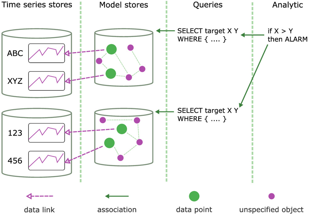
The basic premise of the proposed method, illustrated in Fig. 1, is the abstraction and decoupling of (1) analytics encapsulating the logic for deriving some result time series from a set of input time series, (2) queryable models describing the time series and their contexts, and (3) time-series stores that support the retrieval of input time series with some identifier. The logic of the analytic is expressed once, and multiple queries may connect the analytic to model stores expressed with different technologies and structures in order to find applicable targets. Further, separate queries are associated with the models to retrieve information on the storage of the time series associated with the data points.
The key terminology used in the subsequent sections is now defined. Some of the terms will be described in more detail in subsequent subsections, but a general description is given at this point:
•
An analytic transforms a set of input time series into a result time series. For example, an analytic might convert the temperature setpoint and observed temperature of a room into a series of true/false values indicating whether some error threshold has been crossed.
•
A binding is the connection between an analytic and a particular target to be analyzed. The binding contains information of what data points to use as which named input series in order to evaluate an analytic for a particular target. An analytic can thus be bound to multiple targets, and a particular target, such as a room, may have multiple bound analytics.
•
A data link is the connection between a data point and the actual data store for that point. The link, stored by the model store, associates a data point identifier with a time-series store and a series identifier therein.
•
A data point is the term used for anything that can be observed as a time series, such as sensor observations and control values. It is the same as the Brick schema’s “Point” (Balaji et al. 2018) and RealEstateCore’s “Capability” (Hammar et al. 2019).
•
An information model or model is a description of monitored assets (potential targets for analytics) and related data points. The models are expected to be stored in stores that support some form of querying.
•
A target for an analytic is a physical asset or an abstract entity that is being monitored. Example targets include the spaces in a building, as well as different systems and components such as air handling units and specific sensors.
Assumptions and Requirements
This subsection discusses the assumptions and requirements around the design. The assumptions concern the operating context of the system, i.e., the interfaces of other systems and available information, and the requirements are the architecturally significant requirements for the system itself.
Assumptions about the operating context are enumerated next. For different assumptions, the architecture discussed in this article may not be entirely appropriate, but could be used as a starting point with modifications where applicable:
•
Observation data are available in the form of time series via some API. It should be possible to build an adapter to query the API with an identifier and a pair of timestamps for start and end time. Examples of possible data sources include SQL databases with observations identified by a timestamp and some identifier, Haystack HTTP API, and some BMS cloud services providing access to history data.
•
The information models can be queried for information about the monitored assets and data points. For example, a triple store can store the information of a building using some ontology, and a SPARQL query might be written to, for example, retrieve all air handling units and the data points representing their supply air temperatures and setpoints.
•
The information models contain information about data points’ observation storage. When asked for the information about a data point, the information model should be able to answer that to get the observations for the data point with some identifier, one should query a particular service using some (possibly other, indicated by the model) identifier. In practice, this is used to form a mapping, called a data link, from a particular data point identifier to a tuple containing the identifier for a data store and the identifier used for the data point therein.
•
The model of a building is not updated often. That is, although updates can occur, it is assumed that they are not daily or even weekly events. Updating the model may invalidate cached query results in various systems. Model query results are cached as, for example, SPARQL query times have previously been shown to dominate the overall execution times in similar use cases (Kučera and Pitner 2018).
Given the aforementioned assumptions, the architecturally significant requirements for the system itself include the following:
•
Representing the information of the building is not tied to a specific technology or knowledge model. Given that the information models fulfill the aforementioned assumptions, it should be possible to build adapters to any such model stores.
•
Analytics are run as batches of some days. That is, the architecture is not expected to support streaming analytics nor batches running, for example, every minute. On the other hand, the batches are not expected to be of months or years.
•
An analytic will generally involve up to five variables, instead of tens or hundreds. That is, when evaluating an analytic for a target, there is generally no need to fetch data for more than a handful of variables. The number is a rough heuristic derived by evaluating analytic methods such as Air-Handling Unit Performance Assessment Rules (APAR) (House et al. 2001) and AHU InFO (Bruton et al. 2015).
•
The time-series information is never in a higher resolution than 1 min. That is, when fetching data for a data point for a period 24 h, there will be no more than 1,440 timestamped values.
These requirements form the basis of the architecture presented in the following subsections. The architecture decomposes the application into services, which are described next.
Key Service Descriptions
The functionality is organized into three services that primarily communicate asynchronously via messages on a message bus. Each service may have its own data storage and propagates information to other services via events describing what has happened. Additionally, services react to commands that originate from an user interface or other sources, such as scheduled triggers. The three key services can be summarized as follows:
•
The Analytics service stores the descriptions and definitions of analytics. For each analytic, it also stores the discovered bindings. Finally, the analytics service handles commands to evaluate the analytics for given targets and time ranges, and stores the results.
•
The Models service stores and issues queries against model stores to retrieve (1) bindings between analytics and data points; and (2) data links between data points and time-series stores.
•
The Data Gateway manages the communications with external (time-series) data stores. It provides an endpoint to transform point identifiers into time series for a given time range. It achieves this by communicating with external data sources. The Data Gateway stores the data links that are retrieved from the models. It also stores the connection details for external time-series stores.
Next, the general information flow between the services is described, followed by more detailed descriptions of each key service.
Information Flow between Services
Fig. 2 illustrates the messages—and one query—passed between the services to create, bind, and evaluate an analytic. The contents of the messages are discussed in more detail in the subsequent subsections, but an overview of the intended flow is given at this point. The messages are divided into events and commands. Events, such as AnalyticCreated, are published by services to inform other services that something has happened, and the other services may take some action based on this. Commands, such as CreateAnalytic, are issued to services to request a particular action to be taken. Finally, queries are used to retrieve information from a service.

First, the command AddDataStore (1) is issued against the Data Gateway to register a time-series store with an identifier, for example, a particular HTTP API with an identifier CloudBMS1. This identifier is the one that data links may use to connect a data point to this time-series store. Next, a model store is registered with the AddModelStore command (2), which includes the data link query to find all data links from that model store. This model store could be, for example, a triple store or a relational database, for which adapters would be implemented in the application. Registering the model store causes the data link query to be evaluated, in turn triggering the DataLinksUpdated event (3) carrying the discovered data links.
At some point, an analytic is created by an user with the CreateAnalytic command (4), defining the logic to be evaluated and the variable names that are expected, but not tying it to any particular data. This causes the Analytics service to publish an AnalyticCreated event (5), carrying information about the created analytic, including the input variable names. The Models service listens to the event and stores the variable names for use in validating that the target queries to be connected to that analytic return variables with the same names. Afterward, a target query is added for the analytic to connect it to a model store by issuing the AddTargetQuery command (6) to the Models service. This causes the query to be stored and issued against the model store, for example, as a SPARQL query against a triple store. The query results are parsed and published as AnalyticTargetsUpdated event (7), and the Analytics service stores the bindings from the event. Finally, the analytic is requested to be evaluated for a particular target by issuing the RunAnalyticForTarget (8) command to the Analytics service, causing the service to query the Data Gateway for the data for the bound point identifiers from the GetDataForPoints endpoint (9), and to evaluate the logic.
The next subsections discuss each of the services in more detail. Some important software aspects, such as authentication and authorization, are omitted from the discussion in favor of conciseness. The focus is on the domain of creating, binding, and evaluating analytics.
Analytics
The evaluation logic for an analytic is abstracted as a function that takes in a set of named time series and outputs another time series. Each analytic thus defines a set of variable names that it expects to receive a time series for. The input to an analytic is a mapping of variable names to time series. To give a more concrete example, in the prototype described subsequently, analytics are implemented as Boolean combinations of algebraic expressions in the following form:
These expressions can be parsed to extract the variable names. Further, they can be evaluated with the variables substituted by actual values for a given sample time.
In addition to storing the analytics, the Analytics service stores the discovered bindings for the analytics. The bindings are discovered by the Models service and propagated to the Analytics service by events, which the Analytics service then uses to update the stored bindings. Finally, when an analytic is evaluated for a target, its results are stored by the Analytics service and propagated to other services as events.
In summary, the key commands and events the Analytics service reacts to are the following:
•
CreateAnalytic command containing the details for creating a particular kind of analytic. Will trigger AnalyticCreated on success.
•
RunAnalyticForTarget command containing the identities of the analytic to be run and the target to run it for, as well as the start and end times of the evaluation. Will trigger AnalyticRan on success.
•
AnalyticTargetsUpdated event (described with the Models service in its own subsection) carrying information of discovered bindings for a particular analytic.
The events produced by the Analytics service when reacting to the preceding commands and events are as follows:
•
AnalyticCreated, containing the identifier of the created analytic and the names of the input variables it expects.
•
AnalyticRan, containing the identities of the evaluated analytic and the target, and the result time series from the evaluation.
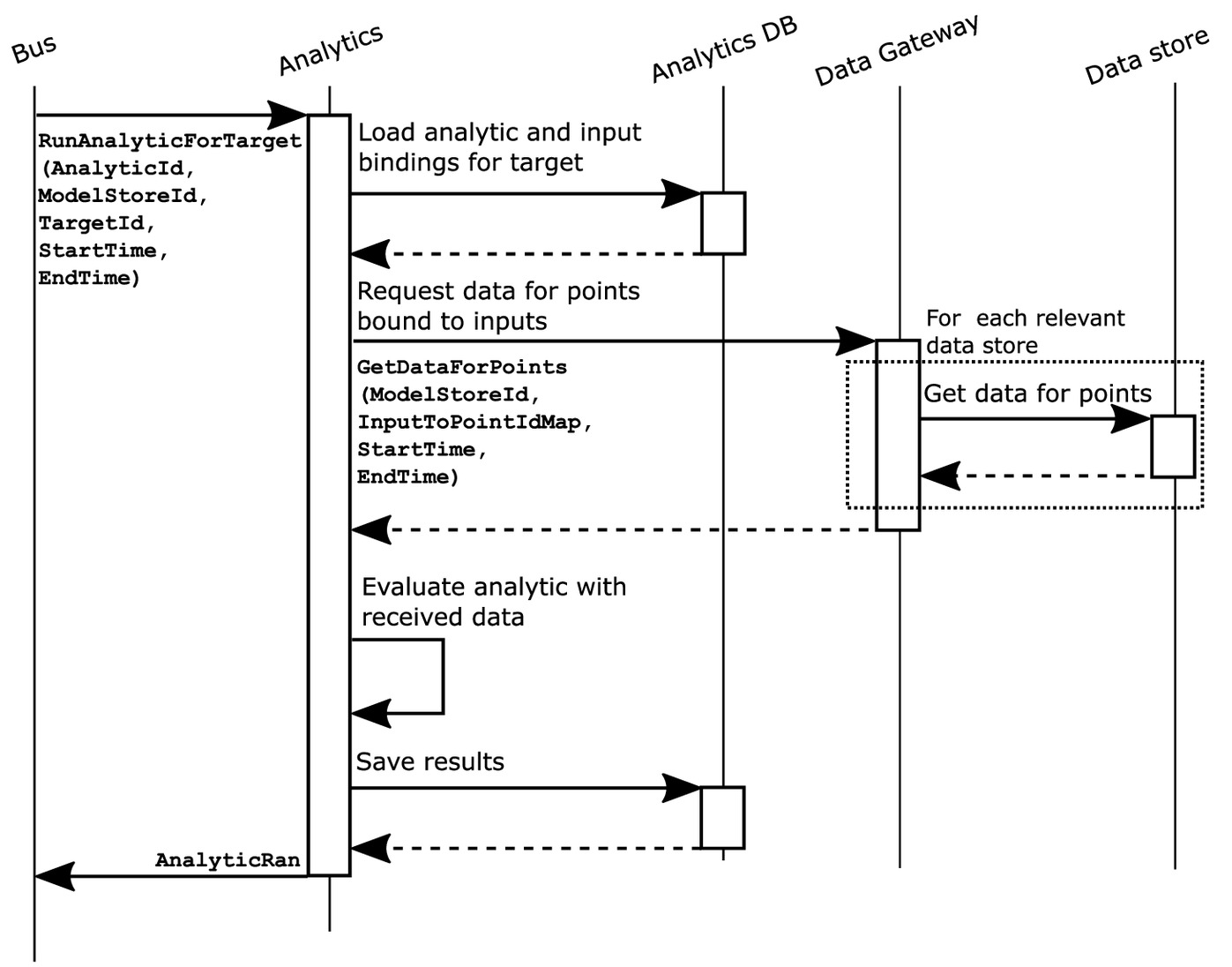
These functionalities cover the core of the Analytics service. Fig. 3 illustrates the flow when the command to evaluate an analytic for a particular binding for a time frame is received. The mappings between analytic input names and point identifiers (InputToPointIdMap) for a particular target, stored from the received AnalyticTargetsUpdated events, are loaded based on the given target identifier (TargetId). The data for relevant data points is requested via the Data Gateway.
Models
The Models service stores the connection information of model stores that can be queried for sets of data point identifiers fulfilling given criteria and also for data links of those data points. The expected interface of the model stores is described next.
First, a model store should be able to process target queries. Target queries are used to find the applicable targets for some analytic, and the point identifiers to associate with variables in the analytic. For example, Fig. 4 shows a partial SPARQL query that could be used to find targets and valid input points for an analytic.
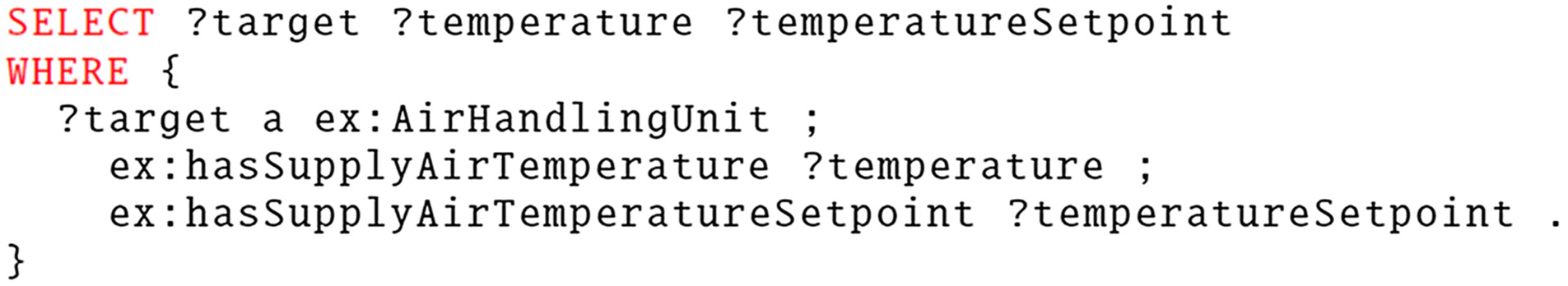
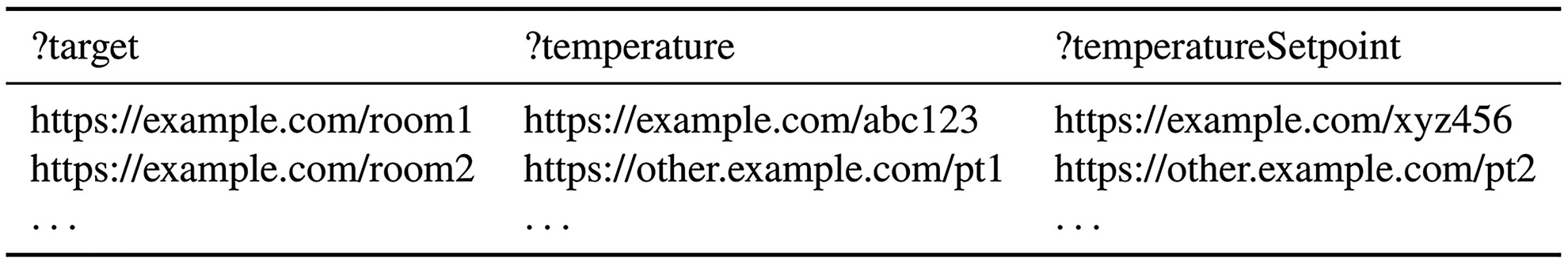
The adapter is built to process the returned variable target as the target identifier, and the rest as variable names from the analytic. This would result in a result set such as shown in Fig. 5. The result set can then be parsed into target bindings, which combine the target identifier and the mapping of input variable names to point identifiers. Importantly, both the target identifiers and point identifiers are assumed unique only within the scope of a particular model store. Thus, in order to fully qualify a target or a data point, the model store identifier needs to also be stored and used.
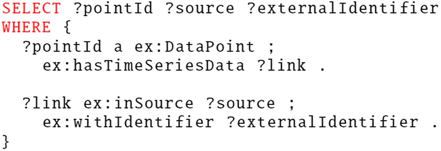
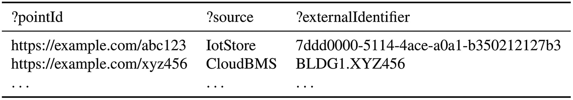
Second, a model store should be able to process data link queries. Data link queries are used to associate a time-series store and an external identifier with data points. A time-series store is some data store that stores the observations related to a data point, such as a BMS API. An external identifier is what the time-series store uses to identify a data point, which may be different than the point identifier used by the model store. Fig. 6 shows a partial SPARQL query that could be used to find data links from a RDF store, resulting in a result set in the shape illustrated in Fig. 7.
Together, the aforementioned capabilities form the basis for mapping sets of data points to analytics and fetching time-series data for the data points. Overall, the Models service reacts to the following commands and events:
•
AddModelStore command for adding a particular kind of model store. Carries a name and connection information that is then stored.
•
AddTargetQuery command carrying identifiers of a model store and an analytic, and the target query to be used to find bindings from the given store for the given analytic. Causes the query to be run and triggers AnalyticTargetsUpdated.
•
AnalyticCreated event carrying the identifier of an analytic and the variable names it expects. The variable names are stored and used to validate target queries added for the analytic return the expected variables.
The events produced by the Models service are as follows:
•
AnalyticTargetsUpdated event triggered when a query is run against a model store. Carries information of the found bindings, i.e., the identifier of the analytic, the model store identifier, and a set of target identifiers with mappings from variable names to point identifiers.
•
DataLinksUpdated event triggered when the query to find data links is run. Carries information of the found data links.
Data Gateway
The Data Gateway fetches data from external time-series stores, for which adapters can be built to fetch data for a set of data points for a given time period. For that purpose, the gateway caches the data links that have been discovered by the Models service and propagated to the gateway via the DataLinksUpdated event. The data links connect each point identifier to a time-series store and an external identifier used for the point in that time-series store.
The Data Gateway requires two primary capabilities to fulfill its role. First, there must exist a way to map time-series store identifiers into concrete implementations for fetching data from those stores. Second is the actual fetching of data for a set of data points from possibly different sources. This is functionally equivalent to what has been called “data adapters” in a previous study (Arjunan et al. 2015).
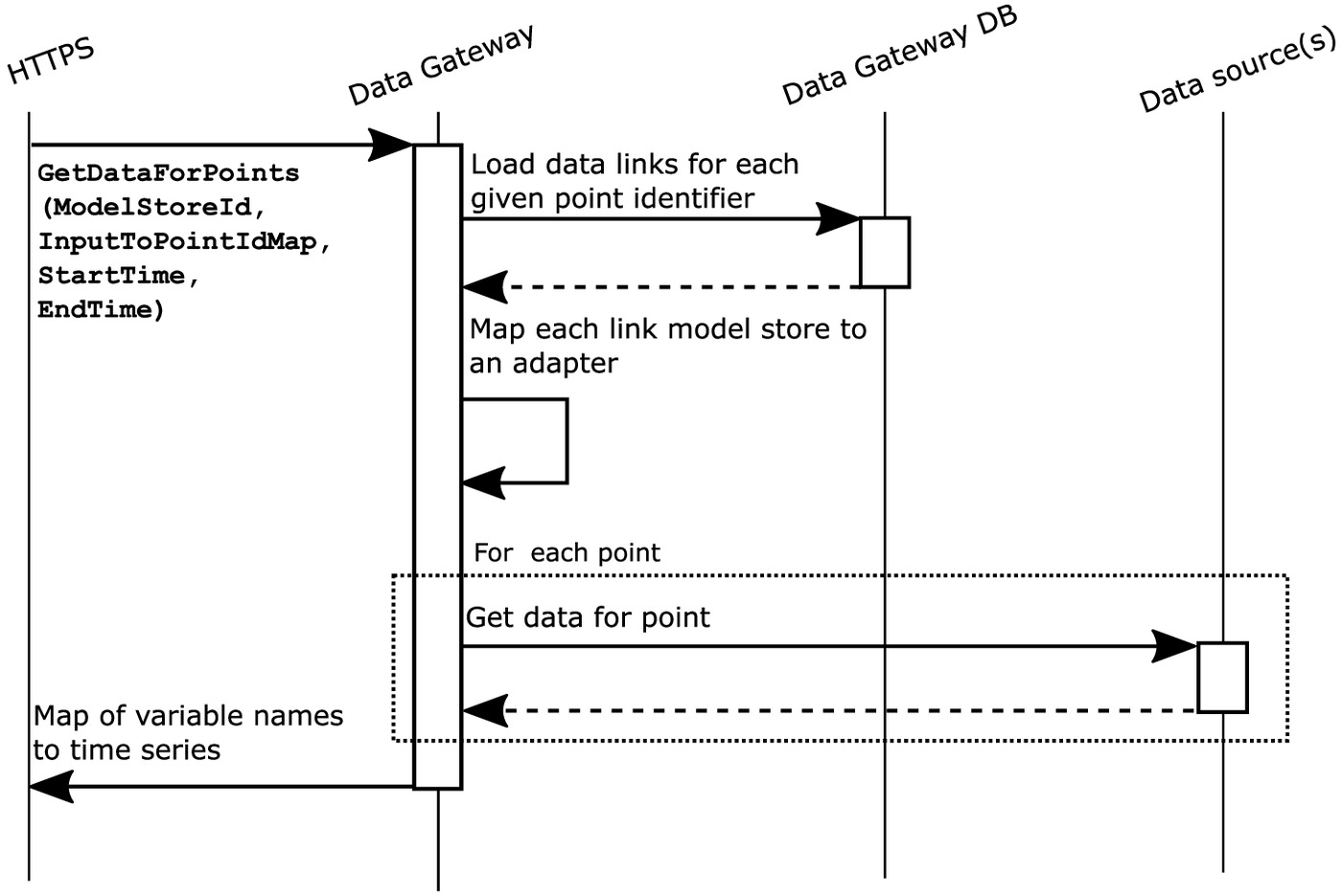
The primary functionality of the Data Gateway is illustrated in Fig. 8. The illustration does not take into account more advanced data fetching strategies, such as grouping data points by their store and batching the requests. Those would be implementation details with no effect to the overall interaction between the services.
The primary requests, commands, and events the Data Gateway reacts to are as follows:
•
AddDataStore command for adding a particular kind of data store. Carries an identifier, type, and connection information that is then stored. Implementations could feasibly exist for adding, for example, SQL databases, or time-series stores.
•
GetDataForPoints request carrying a model store identifier, a map of variable names to point identifiers, and a time frame to fetch the data for. The model store identifier is required to fully qualify the point identifiers, which are assumed unique in the model store scope.
•
DataLinksUpdated event triggered by the Models service. The Data Gateway stores the found data links and uses them when fetching the data.
This concludes the description of the method. In the next section, an example application will be presented.
Application Example: AHU Fault Detection
In order to evaluate and further demonstrate the method, an application prototype is described. In this section, the implementation of a use case is illustrated, including the steps of implementing an analytic, building a model for the target system, and creating queries to bind the data to the analytic.
This section is structured as follows. First, the targeted system and the available data are briefly explained. Next, the implemented analytic is briefly described. Following that, two different models for the same target are explained. Next, the queries connecting the data points described in the models to the analytics are described. Finally, the evaluation of the analytic using the artifacts produced in the previous steps is discussed.
Target System and Data
A published data set of AHU faults (Granderson et al. 2020) was used for the prototype application. The data set contains descriptions and data for a few AHUs. Of these, the simulated data of the second multizone variable air volume AHU data set (MZVAV-2-2.csv) was selected to be modeled and used in testing. The observation data from the data set were imported into a SQLite database.
The target system represents one of three AHUs serving a small commercial building in the US state of Iowa. The AHU has common major components: heating and cooling coils; preheat coil; mixing chamber and dampers for exhaust, outdoor, and recirculated air; and supply and return fans.
The fault data for the AHU include various intensities of stuck outdoor damper, leaking heating coil valve, and stuck cooling coil valve. The data are distributed as short intervals of some days between 2007 and 2009, with most of the days having no data.
Implemented Fault Detection Method: APAR
The APAR (House et al. 2001; Schein et al. 2006) expert rule–based AHU fault detection system was used to illustrate the proposed method. Although subsequent developments have been shown to be more comprehensive and effective (Bruton et al. 2015), the relative simplicity of APAR makes it well-suited for demonstration purposes. APAR describes a set of rules based on energy balances, grouped by the operating mode of the AHU (House et al. 2001; Schein et al. 2006). The rules are expressed as inequalities with user-adjustable parameters.
In the example application, a simple parser for Boolean combinations of inequalities is implemented, and the APAR rules are expressed with that. An example of the expression syntax iswhere variables are prefixed with a question mark. The expressions support basic combinations (AND, OR) of algebraic (addition, subtraction, multiplication, division, and absolute values) inequalities (less than, less than or equal to, greater than, and greater than or equal to).
In the original implementation of APAR, exponentially weighted smoothed averages of the inputs are calculated and stored separately for each state (House et al. 2001). In the prototype implementation, the original input data (Granderson et al. 2020) were resampled to 15-min means.
Because the APAR rules are already expressed as inequalities, their translation to the format at hand is mostly straightforward. For the prototype, the heating mode Rule 1 is implemented. The original rule is defined aswhere = temperature of the air supplied by the AHU, i.e., supply air temperature; = mixed air temperature; = user-defined parameter for air temperature increase over the supply fan; and = user-defined threshold parameter accounting for errors related to temperatures (House et al. 2001).
The rule is used in heating mode to detect inconsistencies in supply air temperature and mixed air temperature, because heating should cause the supply air temperature to be warmer (House et al. 2001). In the implemented expression syntax, the rule can be expressed
The user-defined parameters ?dT_sf and ?e_T are also expressed as variables and not encoded as constants in the expression to enable altering them between targets when reusing the analytic.
APAR groups the rules by the operating mode of the AHU, evaluating only the rules for the current operating mode. Thus, the mode of the system needs to be detected to evaluate the correct rules. Although the simplest way to precondition each rule with a mode check would be to include the mode check in each rule with AND, this has the downside that it complicates changing the mode detection logic due to it being repeated in multiple places. A more scalable approach would be to implement AHU mode checks as separate analytics and have the other analytics depend on those. This potential addition of dependencies between analytics is discussed with other future research directions in the “Discussion” section. However, in favor of simplicity, in the prototype the mode detection and rules are implemented as separate analytics and are expected to be combined when processing the results.
Detecting the mode of operation is implemented with the same kind of inequalities. APAR defines the heating mode such that the supply air temperature is controlled by modulating the heating coil valve, while the cooling coil valve is closed, and the mixing box dampers let in the minimum outdoor air (House et al. 2001). In the implementation, the mixing box damper positions are ignored, and instead the focus is on the occupancy status and the positions of the heating and cooling coil valves. The inequality for detecting heating mode is then implemented as follows:where ?occ = occupancy status (0 = unoccupied and 1 = occupied); ?u_hc = control signal of the heating coil; and ?u_cc = control signal of the cooling coil. The binary occupancy status is converted into a floating point number in the analytic implementation, which is why the inequality compares against 0.01 to avoid problems with imprecision. The assumption here is that the control signals vary from 0.0 (fully closed) to 1.0 (fully open) and that occupancy is indicated with a zero or one. Normalization of numeric values and units is another potential future research direction, also discussed subsequently.
Implementing the Models
Web Ontology Language (OWL) ontologies and RDF triple store were chosen as the technology stack for expressing and storing the models. For the purposes of the application example, the AHUs are described as RDF triples with two different modeling approaches and stored in a GraphDB triple store. This subsection explains two approaches to modeling the terminological (TBox) and assertional (ABox) knowledge required to support the analytics example. The methods of developing ontologies are discussed elsewhere (for example, Suárez-Figueroa et al. 2012), and are not the focus of this study. Thus, this section will only briefly introduce the example TBox and ABox models.
The TBox and ABox are both added to a GraphDB repository to form the knowledge base. It is worth reiterating that using OWL ontologies and triple stores is not required by the method, but is one possible choice among others. For example, the information could similarly be stored in a relational database and queried with SQL. However, as discussed in the “Related Work” section, using ontologies and OBDA offers flexibility and richer semantics over encoding models in relational database schemas.
Two models with different ontologies forming the TBoxes are created as examples. First, a model using Brick schema (Balaji et al. 2018) is explained. Following that, another modeling approach based on flow systems ontology (FSO) (Kukkonen et al. 2022) is explained. The prefixes used are listed in Fig. 9. The full models are available online (Kukkonen 2022). As the purpose of the models is to only demonstrate that models with different modeling approaches can be connected to the analytic, their specific contents and preparation steps are not discussed in detail.

Brick Schema
Brick is an ontology for describing the assets and their relationships in buildings, including logical and virtual assets such as data points. Full documentation of Brick is available online (Brick Consortium 2021) and thus not repeated here. For the context at hand, the relevant subset of the ontology consists of
•
brick:hasPart/brick:isPartOf for (de)composition of objects;
•
brick:hasPoint/brick:isPointOf for assigning points to assets;
•
subclasses of brick:Point, such as brick:Valve_Command, for classifying data points;
•
subclasses of brick:Equipment, such as brick:AHU, for classifying assets; and
•
brick:timeseries, as well as brick:hasTimeseriesId and brick:storedAt for defining data links for points.
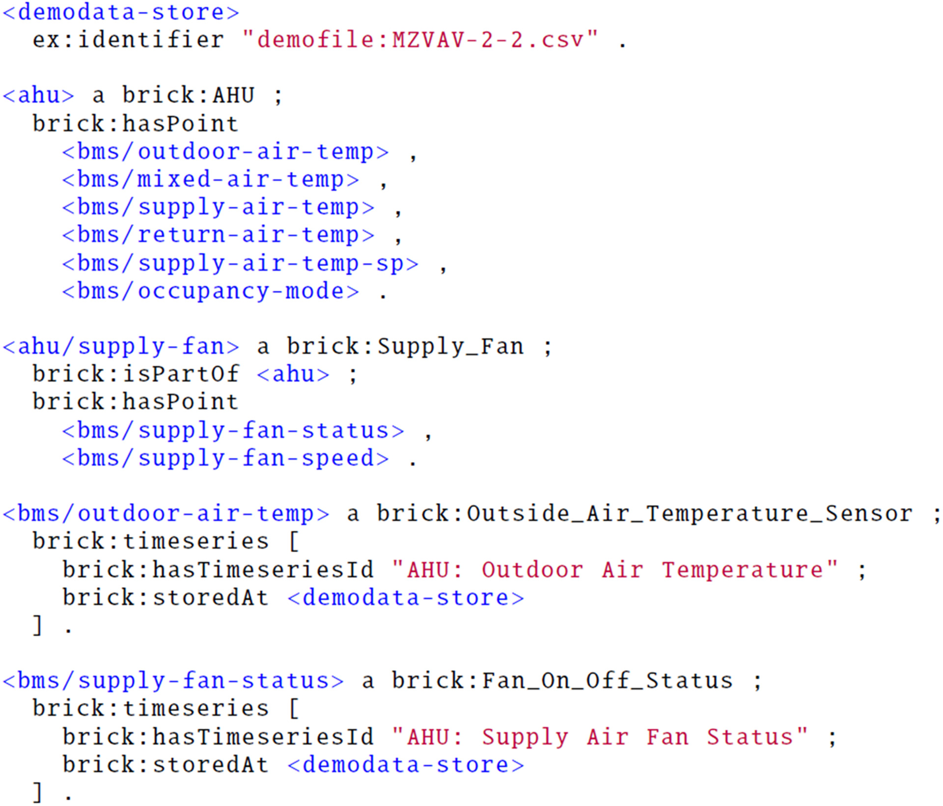
A subset of the assertional model is shown in Fig. 10. In brief, the data points are assigned either directly to the AHU or to one of its subcomponents. The data points are classified with the available classes and connected to their storage with brick:timeseries properties. Resources connected with brick:storedAt are nonnormative, and in this example, a simple string property is used to identify the time-series store as demofile with a particular name. Data Gateway has an adapter for accessing the data in SQLite database based on the file name and the column name.
FSO-Based Approach
As an alternative to the tagging approach of Brick, another model is implemented with a different paradigm. For example, whereas Rule 1 uses the term mixed air temperature, what it actually requires is the temperature before the heating and cooling coils. In AHUs with no mixing chamber and thus no mixed air, this rule is still applicable. The alternative modeling approach stems from using relationships of components and simplified assertions stating that points are before, within, or after components.
The alternative model combines the FSO (Kukkonen et al. 2022) and an unnamed data point ontology that connects data points to components (Kukkonen 2021). Because complete descriptions are available elsewhere, only a brief overview of the terminology is provided here. Although ontology engineering best practices would call for reusing or aligning existing ontologies, such as Brick, the purpose here of using different ontologies is to demonstrate the method’s ability to bind analytics to data points through different kinds of models. As such, the used ontology is not necessarily something that should be used in further applications, but it serves to demonstrate a sufficiently different model. Developing a proper ontology combining FSO with data points and potentially reusing or aligning parts of Brick is outside of the scope of this study.
FSO contains the vocabulary to assert mass and flow relationships between components and systems, as well as a component classification derived from IFC. The fso:System can also be decomposed into subsystems, and even more particularly to supply and return systems.
The data point ontology has classes for sensors, setpoints, and such, as well as the relationships to assert their position relative to components. The relationships include data:hasSupplySensor, data:hasDischargeSensor, and data:hasControl.
Although brick:timeseries could again be used for data links, another approach is implemented for the sake of demonstration. A simple hasDataLink property is used, where the resource then hasSource and hasExternalIdentifier.
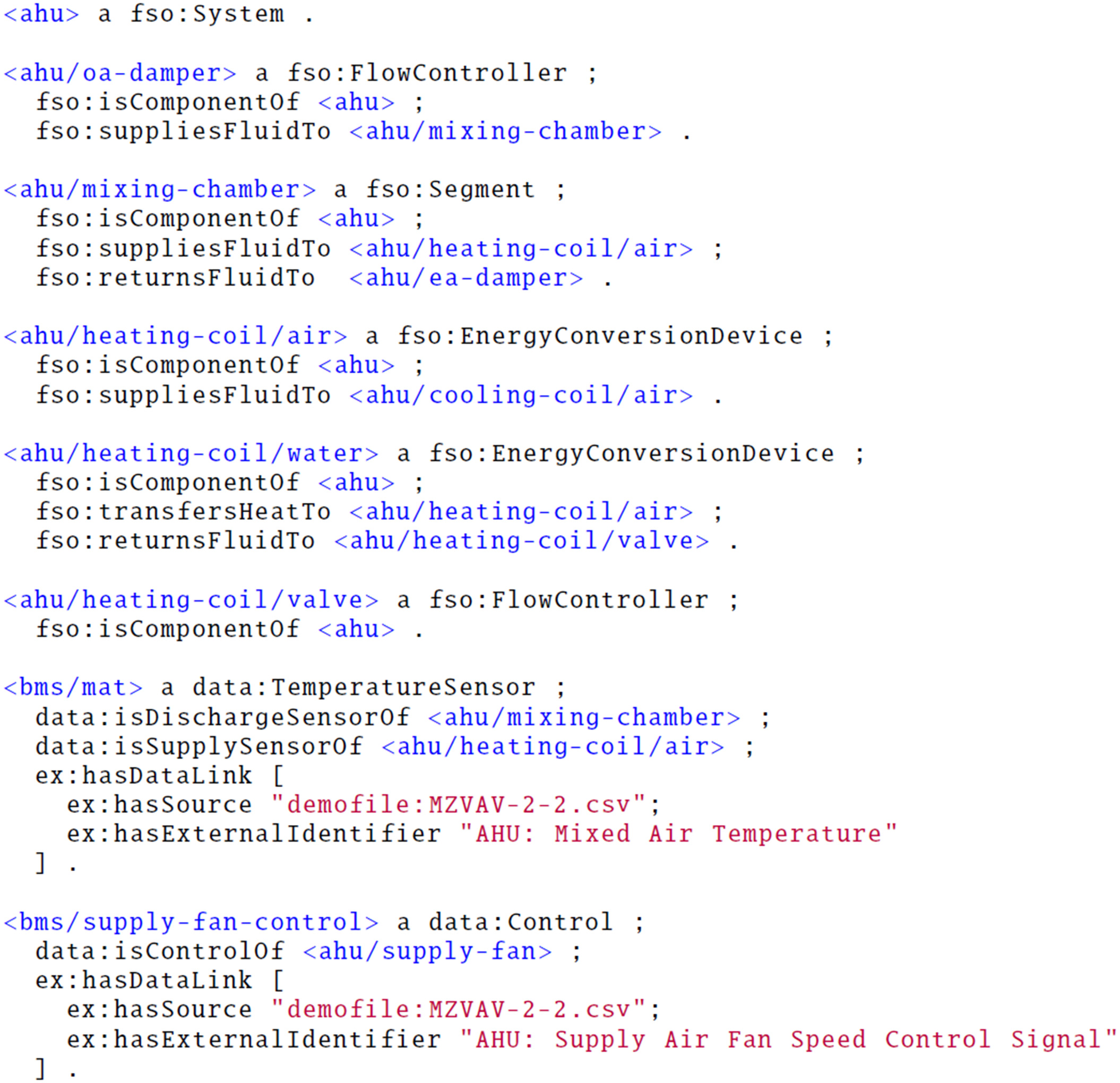
Fig. 11 shows a fragment of the alternative assertional model. To summarize, the AHU is modeled as a fso:System consisting of the various components, which have their air and heat flow relationships asserted. The data points are connected to the components.
APAR Parameters
APAR rules have user-defined parameters that are intended to be adjusted to fit a particular system. In the case of the example rule, there are two: (or ?dT_sf), which is intended to account for the estimated air temperature increase over the supply fan, and (or ?e_t), which is intended to account for errors related to temperature measurements.
Implementing these parameters could be done in multiple ways. For the purpose of the example, the parameters are implemented as follows. Each target may have parameters bound with properties in an example apar namespace. The object of the property is a data point like any other. The data links are defined against a store that returns constant values parsed from the external identifier of the data link. An example is shown as a Turtle excerpt in Fig. 12.
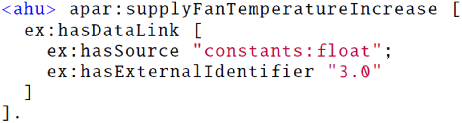
The external identifier in this case has special handling by the data store handler registered for time-series stores matching the regular expression constants:(.*), where anything after the string constants: is interpreted as the value type. For example, linking a data point to a time-series store constants:float will cause the identifier to be interpreted as a float. Thus, when the example data link in Fig. 12 is used to retrieve data through the Data Gateway, the handler will parse the identifier (“3.0”) as a float in this case, and return the constant value with 1-min sample rate for the requested time frame.
Finally, to account for targets that do not have a particular parameter defined, the target queries for the rules can use default values, as will be shown in the next subsection. These are predefined data links that are shared between all the targets.
Connecting Analytics to Data with Queries
SPARQL queries to connect the data to the analytics are shown here, and the full set is available online along with the models (Kukkonen 2022). The used prefixes are shown in Fig. 9.
Two kinds of queries are defined. First, the query to retrieve data links from a store is defined. It is not particular to any analytic, but is related to the model store. Second, an example target query for finding applicable targets and their variable bindings is illustrated.
Brick Schema
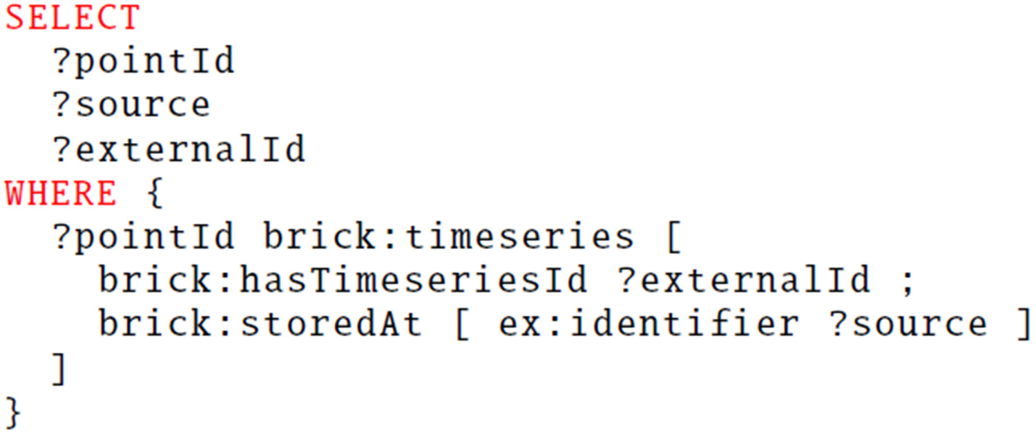
The data link query for Brick schema is shown in Fig. 13. It traverses the properties brick:timeseries, brick:hasTimeseriesId, and brick:storedAt to get a result set connecting the internationalized resource identifier (IRI) of the point as the point identifier, store identifier, and the external identifier for the point.
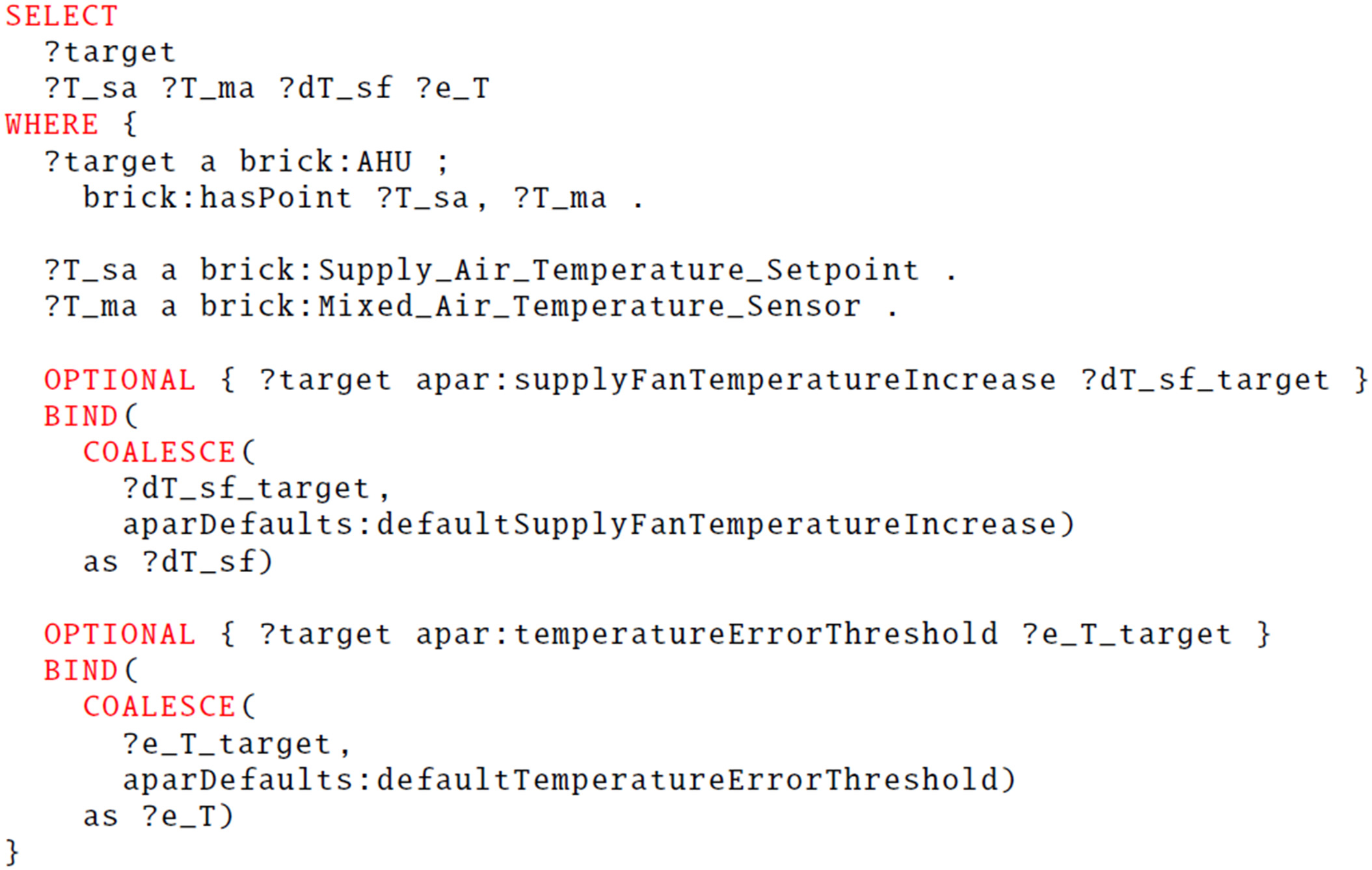
The query used to find the bindings for APAR rule 1 from the Brick model is shown in Fig. 14. Because Brick relies heavily on the classification of points, the query is primarily about the classes of points. The used pattern finds points of certain classes that are the points of an air handling unit. Additionally, the APAR user parameters are optionally retrieved if defined, with a default fallback if a parameter is not defined for a particular target. The parameter binding is the same as in the FSO-based approach because it is not dependent on either Brick or FSO but is an APAR-specific addition. Here, the aparDefaults are expected to be stored in the same triple store as the queried information models, but they could alternatively be queried from other sources with, for example, federated queries.
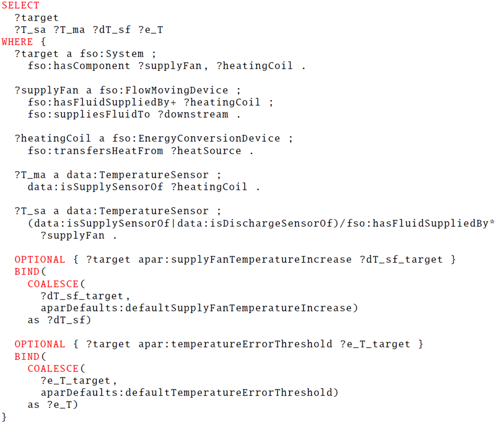
FSO-Based Approach
The data link query for the FSO-based approach is shown in Fig. 15. It is very similar to the one used for Brick schema in the previous subsection.
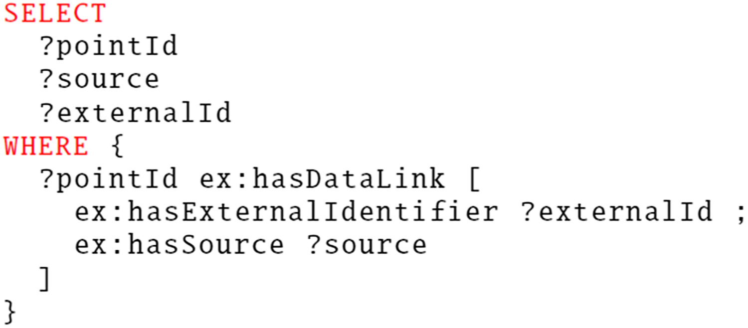
The target query for the FSO-based approach is shown in Fig. 16. Using component connections and not relying on the detailed point taxonomy of Brick yields a slightly more complicated query for this use case. The supply air temperature is defined as the temperature point of a component downstream of the supply fan, and the supply fan itself is defined as a fan inside the AHU that supplies fluid (air) to some other component. The mixed air temperature is defined as the temperature point before the heating coil, where the heating coil is an energy conversion device that has heat transferred from some other component.
Evaluating the Rule
The overall flow of evaluating an analytic was described in the “Information Flow between Services” section, but is repeated here with a more concrete example. When the Analytics service receives the command to evaluate an analytic, the command carries the ID of the analytic, identifiers for the model store and target that together uniquely identify the target, and the start and end timestamps to run the analytic for. With this information, the Analytics service can retrieve the analytic logic from the database and deserialize it into executable form, and also read the variable bindings for the given analytic and target. These variable bindings are passed on to Data Gateway, which in turn has stored the data links for the points. The data links identify the time-series store and the ID to use when querying that store to retrieve data for a given point. In this case, most of the data is retrieved from a local SQLite database, and the constants are generated as requested. After the Data Gateway responds to the Analytics service, the service has all it needs to evaluate the analytic: the analytic logic, and a set of named time series to pass in as inputs for the logic. The analytic is then evaluated against the inputs, and the result is stored.
Discussion
The limited example prototype showcased in this paper illustrates a simplified process of using the proposed method to implement an expert rule–based fault detection application. For a more structured approach of designing applications and capturing their knowledge requirements, methods such as presented by Schneider et al. (2020) exist. The focus of this study is a more detailed and structured definition of the key services and their interactions for utilizing queries and information models. The goal is to enable the analytics logic and possible downstream processing to be implemented centrally, while enabling queries on various models in different query languages to connect data points to the analytics.
Although the asynchronous message-based communication between the services makes some of the communication patterns more complex and causes the need to cache some information, it also greatly simplifies the horizontal scaling of the services. For example, multiple instances of Data Gateway could handle requests for time-series data, and each would use cached information about data links instead of issuing queries against the information models. On the other hand, the cached information needs to be updated somehow, which was not explored in this study. Cache management has strong ties to overall model management and provenance, which itself is an important future research direction: how and when are information models updated, and how is that information propagated to relevant services.
Limitations of the proposed method and architecture include a lack of data point aggregations, such as the average of all temperature sensors matching a pattern. Instead, the analytics are expected to operate on a set of specific, named inputs of one time series each. Further, the current approach does not consider reusing queries: if two model stores using, for example, Brick are connected, both would require new queries to be instantiated to connect analytics, leading to duplication.
Potential future work identified includes the study of enabling dependencies between analytics, where the output of one analytic could be used as the input for another analytic. This could prove useful for avoiding repetitions of shared logic, such as state identification as used in APAR. Other major area of future development is approaches into describing and normalizing values and units of inputs. For example, control signals may be expressed with a decimal between zero and one or as integers ranging from 0 to 100. Further, the example used in this study is limited to a data set from one building, and exploring the scalability to further buildings is an important future research direction. Finally, supporting the training and use of machine learning models for analytics is another potential future research direction.
As discussed by Kučera and Pitner (2018), applying analytics does not need to be all or nothing, but a monitoring solution can be built use case by use case. In a similar manner, information models for plugging time-series stores into centralized analytics suites can be developed depending on the available existing digital information and budget. However, care should be taken and lessons learned from previous knowledge modeling experiences in order to build simple models that can be grown into more complex ones, instead of needing to be replaced entirely when more complex use cases are desired.
Conclusion
Given that significant amounts of energy are wasted in the operation of buildings, the application of analytics supporting MBCx is limited. This study reviewed the varying approaches used to connect building data observations to analytics and showed that a structured method using technology-independent information models has not been discussed. To address this, a method was described for using structured descriptions of building systems in queryable stores to bind inputs to time-series analytics. The method was described through a software architecture and evaluated with an example prototype of two air handling unit models and a fault detection expert rule. The process of modeling the target systems and defining queries to connect the analytic to the data stores was walked through.
The method was shown to support connecting a time-series transformer to two very different models of the air handling unit. The method enables the analytic logic to be expressed once and bound to different data points, supporting scalability in a centralized monitoring solution. Further research topics were identified, including dependencies between analytics, considering units of measurement, and integrating machine learning model training and utilization.
Although no widely used industry standard exists for describing the data points of building systems in the kind of context required by many analytics applications, the described method is a potential approach to building centralized monitoring applications that can support different information models.
Data Availability Statement
Some or all data, models, or code generated or used during the study are available in a repository or online in accordance with funder data retention policies. The AHU data were from Granderson et al. (2020), available at https://doi.org/10.1038/s41597-020-0398-6. The example ontologies, triples, and queries are available at https://doi.org/10.5281/zenodo.7361351 (Kukkonen 2022).
Acknowledgments
This work was supported by the K.V. Lindholm Foundation.
References
Ahmed, A., J. Ploennigs, K. Menzel, and B. Cahill. 2010. “Multi-dimensional building performance data management for continuous commissioning.” Adv. Eng. Inf. 24 (4): 466–475. https://doi.org/10.1016/j.aei.2010.06.007.
Arjunan, P., M. Srivastava, A. Singh, and P. Singh. 2015. “OpenBAN: An open building analytics middleware for smart buildings.” In Proc., 12th EAI Int. Conf. on Mobile and Ubiquitous Systems: Computing, Networking and Services (MOBIQ–UITOUS’15), 70–79. Brussels, Belgium: Institute for Computer Sciences, Social-Informatics, and Telecommunications Engineering.
Balaji, B., et al. 2018. “Brick: Metadata schema for portable smart building applications.” Appl. Energy 226 (Sep): 1273–1292. https://doi.org/10.1016/j.apenergy.2018.02.091.
Brick Consortium. 2021. “Introduction—Brick ontology documentation.” Accessed December 22, 2022. https://docs.brickschema.org/intro.html.
Bruton, K., D. Coakley, P. Raftery, D. O. Cusack, M. M. Keane, and D. T. O’Sullivan. 2015. “Comparative analysis of the AHU InFO fault detection and diagnostic expert tool for AHUs with APAR.” Energy Effic. 8 (Apr): 299–322. https://doi.org/10.1007/s12053-014-9289-z.
Bruton, K., P. Raftery, P. O’Donovan, N. Aughney, M. M. Keane, and D. T. O’Sullivan. 2014. “Development and alpha testing of a cloud based automated fault detection and diagnosis tool for air handling units.” Autom. Constr. 39 (Apr): 70–83. https://doi.org/10.1016/j.autcon.2013.12.006.
Cao, X., X. Dai, and J. Liu. 2016. “Building energy-consumption status worldwide and the state-of-the-art technologies for zero-energy buildings during the past decade.” Energy Build. 128 (Sep): 198–213. https://doi.org/10.1016/j.enbuild.2016.06.089.
Fierro, G., et al. 2019. “Mortar: An open testbed for portable building analytics.” ACM Trans. Sens. Networks 16 (1): 1–31. https://doi.org/10.1145/3366375.
Granderson, J., G. Lin, A. Harding, P. Im, and Y. Chen. 2020. “Building fault detection data to aid diagnostic algorithm creation and performance testing.” Sci. Data 7 (1): 65. https://doi.org/10.1038/s41597-020-0398-6.
Gunay, H. B., W. Shen, and G. Newsham. 2019. “Data analytics to improve building performance: A critical review.” Autom. Constr. 97 (Jan): 96–109. https://doi.org/10.1016/j.autcon.2018.10.020.
Hammar, K., E. O. Wallin, P. Karlberg, and D. Hälleberg. 2019. “The realestatecore ontology.” In Proc., Semantic Web–ISWC 2019: 18th Int. Semantic Web Conf., 130–145. Auckland, New Zealand: Springer.
Harris, N., T. Shealy, H. Kramer, J. Granderson, and G. Reichard. 2018. “A framework for monitoring-based commissioning: Identifying variables that act as barriers and enablers to the process.” Energy Build. 168 (Jun): 331–346. https://doi.org/10.1016/j.enbuild.2018.03.033.
House, J. M., H. Vaezi-Nejad, and J. M. Whitcomb. 2001. “An expert rule set for fault detection in air-handling units.” ASHRAE Trans. 107: 858–871.
Hu, S., E. Corry, E. Curry, W. J. Turner, and J. O’Donnell. 2016. “Building performance optimisation: A hybrid architecture for the integration of contextual information and time-series data.” Autom. Constr. 70 (Oct): 51–61. https://doi.org/10.1016/j.autcon.2016.05.018.
Hu, S., E. Corry, M. Horrigan, C. Hoare, M. Dos Reis, and J. O’Donnell. 2018. “Building performance evaluation using OpenMath and Linked Data.” Energy Build. 174 (Sep): 484–494. https://doi.org/10.1016/j.enbuild.2018.07.007.
Hu, S., J. Wang, C. Hoare, Y. Li, P. Pauwels, and J. O’Donnell. 2021. “Building energy performance assessment using linked data and cross-domain semantic reasoning.” Autom. Constr. 124 (Apr): 103580. https://doi.org/10.1016/j.autcon.2021.103580.
Kim, W., and S. Katipamula. 2018. “A review of fault detection and diagnostics methods for building systems.” Sci. Technol. Built Environ. 24 (1): 3–21. https://doi.org/10.1080/23744731.2017.1318008.
Kramer, H., G. Lin, C. Curtin, E. Crowe, and J. Granderson. 2020. “Building analytics and monitoring-based commissioning: Industry practice, costs, and savings.” Energy Effic. 13 (3): 537–549. https://doi.org/10.1007/s12053-019-09790-2.
Kučera, A., and T. Pitner. 2018. “Semantic BMS: Allowing usage of building automation data in facility benchmarking.” Adv. Eng. Inf. 35 (Jan): 69–84. https://doi.org/10.1016/j.aei.2018.01.002.
Kukkonen, V. 2021. “Semantic contextualization of BAS data points for scalable HVAC monitoring.” In Proc., ECPPM 2021–eWork and eBusiness in Architecture, Engineering and Construction: Proc., 13th European Conf. on Product & Process Modelling (ECPPM 2021). Boca Raton, FL: CRC Press.
Kukkonen, V. 2022. “RDF models and SPARQL queries for decoupled analytics demonstration.” Zenodo, November 25, 2022.
Kukkonen, V., A. Kücükavci, M. Seidenschnur, M. H. Rasmussen, K. M. Smith, and C. A. Hviid. 2022. “An ontology to support flow system descriptions from design to operation of buildings.” Autom. Constr. 134 (Feb): 104067. https://doi.org/10.1016/j.autcon.2021.104067.
Lin, G., H. Kramer, V. Nibler, E. Crowe, and J. Granderson. 2022. “Building analytics tool deployment at scale: Benefits, costs, and deployment practices.” Energies 15 (13): 4858. https://doi.org/10.3390/en15134858.
Lork, C., V. Choudhary, N. U. Hassan, W. Tushar, C. Yuen, B. K. Ng, X. Wang, and X. Liu. 2019. “An ontology-based framework for building energy management with IoT.” Electronics 8 (5): 485. https://doi.org/10.3390/electronics8050485.
Marinakis, V. 2020. “Big data for energy management and energy-efficient buildings.” Energies 13 (7): 1555. https://doi.org/10.3390/en13071555.
NIST. 2021. “Semantic interoperability for building data.” Accessed March 21, 2023. https://www.nist.gov/programs-projects/semantic-interoperability-building-data.
Pau, M., P. Kapsalis, Z. Pan, G. Korbakis, D. Pellegrino, and A. Monti. 2022. “MATRYCS—A big data architecture for advanced services in the building domain.” Energies 15 (7): 2568. https://doi.org/10.3390/en15072568.
Project Haystack. 2022. “Project Haystack.” Accessed June 27, 2022. https://project-haystack.org/.
Quinn, C., A. Z. Shabestari, T. Misic, S. Gilani, M. Litoiu, and J. J. McArthur. 2020. “Building automation system—BIM integration using a linked data structure.” Autom. Constr. 118 (Oct): 103257. https://doi.org/10.1016/j.autcon.2020.103257.
Ramprasad, B., J. McArthur, M. Fokaefs, C. Barna, M. Damm, and M. Litoiu. 2018. “Leveraging existing sensor networks as IoT devices for smart buildings.” In Proc., 2018 IEEE 4th World Forum on Internet of Things (WF-IoT), 452–457. New York: IEEE.
Schein, J., S. T. Bushby, N. S. Castro, and J. M. House. 2006. “A rule-based fault detection method for air handling units.” Energy Build. 38 (12): 1485–1492. https://doi.org/10.1016/j.enbuild.2006.04.014.
Schneider, G. F., et al. 2020. “Design of knowledge-based systems for automated deployment of building management services.” Autom. Constr. 119 (Nov): 103402. https://doi.org/10.1016/j.autcon.2020.103402.
Schneider, G. F., Y. Kalantari, G. Kontes, S. Steiger, and D. V. Rovas. 2016. “An ontology-based tool for automated configuration and deployment of technical building management services.” In Proc., CESBP–Central European Symp. on Building Physics/BauSIM 2016. Dublin, Ireland: International Group for Lean Construction.
Schneider, G. F., Y. Kalantari, G. D. Kontes, G. Grün, and S. Steiger. 2017. “A platform for automated technical building management services using ontology.” In Proc., Lean and Computing in Construction Congress—Volume 1: Proc., Joint Conf. on Computing in Construction, 321–328. Heraklion, Greece: Heriot-Watt Univ.
SkyFoundry. 2023. “Product—SkyFoundry.” Accessed March 21, 2023. https://skyfoundry.com/product.
Suárez-Figueroa, M. C., A. Gómez-Pérez, E. Motta, and A. Gangemi. 2012. Ontology engineering in a networked world. Berlin: Springer.
Tamani, N., S. Ahvar, G. Santos, B. Istasse, I. Praca, P. E. Brun, Y. Ghamri, N. Crespi, and A. Becue. 2018. “Rule-based model for smart building supervision and management.” In Proc., 2018 IEEE Int. Conf. on Services Computing (SCC), 9–16. New York: IEEE.
Wang, W., M. R. Brambley, W. Kim, S. Somasundaram, and A. J. Stevens. 2018. “Automated point mapping for building control systems: Recent advances and future research needs.” Autom. Constr. 85 (Jan): 107–123. https://doi.org/10.1016/j.autcon.2017.09.013.
Information & Authors
Information
Published In

Journal of Computing in Civil Engineering
Volume 37 • Issue 6 • November 2023
Copyright
This work is made available under the terms of the Creative Commons Attribution 4.0 International license, https://creativecommons.org/licenses/by/4.0/.
History
Received: Jan 18, 2023
Accepted: Jun 8, 2023
Published online: Aug 22, 2023
Published in print: Nov 1, 2023
Discussion open until: Jan 22, 2024
ASCE Technical Topics:
- Architectural engineering
- Artificial intelligence and machine learning
- Building systems
- Buildings
- Computer programming
- Computing in civil engineering
- Construction engineering
- Construction methods
- Continuum mechanics
- Data analysis
- Deformation (mechanics)
- Detection methods
- Energy methods
- Engineering fundamentals
- Engineering mechanics
- Expert systems
- HVAC
- Methodology (by type)
- Research methods (by type)
- Smart buildings
- Solid mechanics
- Structural engineering
- Structural mechanics
- Structures (by type)
Authors
Metrics & Citations
Metrics
Citations
Download citation
If you have the appropriate software installed, you can download article citation data to the citation manager of your choice. Simply select your manager software from the list below and click Download.