Convoluted Reciprocity and Other Methods for Vehicle Speed Estimation in Bridge Weigh-in-Motion Systems
Publication: Journal of Bridge Engineering
Volume 29, Issue 2
Abstract
In bridge weigh-in-motion systems, the vehicle speed is a fundamental input parameter for the weighing algorithm. The speed is generally obtained by processing structural responses measured at different locations along the bridge length. For this purpose, the convoluted reciprocity relationship was derived and utilized as the basis for a novel speed estimation method. In addition, this document reviewed other existing methods, such as correlation or point load approximation methods, using exclusively measured strain signals from the soffit of a bridge. These methods were studied and compared with illustrative examples and parametric studies based on simulated vehicle–bridge interaction responses. As a result, this document proposed several new possibilities for speed estimation. Subsequently, these methods were validated empirically with responses from a scaled experiment. The results clearly showed that the new speed estimation strategies proposed in this work offer a significant improvement in accuracy compared to existing methods.
Introduction
A bridge weigh-in-motion (BWIM) system is an installation to weigh vehicles that cross a bridge traveling at normal operational traffic speeds. The weighing operation is based on measured structural responses that are processed to estimate the vehicle speed, axle geometry, individual axle weights, and total gross vehicle weight. Compared to pavement-based weigh-in-motion systems, where the instrumentation is integrated into the bituminous layer, BWIM systems generally offer a more convenient and durable solution because the required sensors are installed on the soffit of the bridge, an operation that does not disrupt the traffic (van Loo and Žnidarič 2019; Stawska et al. 2021). In addition, because the weight estimation process is based on longer signals (the bridge response), the method can provide good accuracies (OBrien and Žnidarič 2001; Jacob et al. 2002). BWIM technology was originally proposed in the 1970s and has regained interest in the last decade, evidenced by the abundance of recent state-of-the-art reviews found in Bakht and Mufti (2015), Lydon et al. (2016), Yu et al. (2016), Žnidarič et al. (2018), and Debojyoti and Koushik (2023).
A typical BWIM installation system uses strain signals that are often measured by means of transducers or directly with strain gauges attached to the bridge soffit (Žnidarič et al. 2018). The location of the weighing sensors is generally at the section of maximum strain response (midspan) in the longitudinal direction. In the transverse direction, they are located at multiple points across the section, and their signals are added together for the standard BWIM algorithm. Alternatively, the different signals in the transverse direction can be processed with the less common and more challenging 2D BWIM algorithm (Žnidarič et al. 2018). It is worth noting that it is also possible to define BWIM installations based on other measured load effects, such as vertical deformations (Ojio et al. 2016), rotations (Huseynov et al. 2022), and even to some extent with accelerations (OBrien et al. 2020).
After sensor installation, the BWIM system needs to be calibrated. This is done with calibration trucks of known weight and speed (OBrien et al. 2006) or with free-running traffic combined with nonlinear optimization (Žnidarič et al. 2018). At the end of the calibration process, the influence lines (ILs) for all weighing sensors are available, which are essential elements in the BWIM algorithm (Moses 1979). During normal operation of the weighing system, additional information about each vehicle is required, namely, their speed, number of axles, and the distances between them. This information is obtained by processing the signals from additional sensors.
Early in BWIM technology, speed and axle detectors were mounted on the pavement near the bridge ends, which produced traffic disruptions and suffered from durability issues. However, this was eventually replaced with alternative solutions that rely exclusively on sensors mounted on the bridge soffit, called FAD (free of axle detectors) or NOR (nothing on the road) solutions introduced by the WAVE project (OBrien and Žnidarič 2001). The additional sensors required for FAD and NOR are normally located at one-quarter and three-quarters of the span or on secondary elements that have relatively shorter influence lines and feature sharp peaks (Kalin et al. 2006).
A BWIM system needs to estimate first the speed of any passing vehicle before proceeding to its axle identification and final weight calculation. Therefore, speed estimation is a fundamental step to accurate vehicle weighing. The identification of the vehicle’s speed from global strain signals is difficult (Yu et al. 2016) because the measured responses usually do not have distinctive sharp features. In addition, the measured responses include structural dynamic components and are corrupted by noise. Speed estimation must be achieved without prior knowledge of the vehicle properties and its axle configuration. This is why, ideally, the signals used for speed estimation should have distinct peaks corresponding to each axle of the vehicle. However, this is not always possible because of the structural configuration of the bridge. Different strategies and methods have been proposed to solve this problem, which are reviewed in the following section. Note that this document refers to speed as the magnitude of the vehicle’s velocity, whereas velocity also describes its direction of forward motion.
Review of Existing Speed Estimation Methods
The initial and simplest idea to identify the vehicle’s speed was to study the peaks on the measured signals. The time delay between peaks in signals at separate locations, together with the actual distance between them, provides an estimate of the event’s speed (Liljencrantz et al. 2007), an idea that has also been termed peak-to-peak (OBrien and Žnidarič 2001). However, this was quickly adopted only as a reasonable first guess. Kalhori et al. (2017) clearly showed, with laboratory and field tests, that the peak-to-peak approach did not provide acceptable speed estimates. Others have tried to improve the idea by automating peak detection using wavelets (Chatterjee et al. 2006; Kalin et al. 2006). The peak-to-peak approach was reported to be adequate for BWIM installations on orthotropic bridges of 6–10 m span lengths (OBrien and Žnidarič 2001). However, this is not the case for longer bridges or bridges with thick slabs (Kalhori et al. 2017).
Arguably, the most common method to estimate speed is calculating the cross-correlation (or simply correlation) between signals measured at two different sections in the longitudinal direction (Yu et al. 2016). The speed is estimated by the distance between sensors divided over the time lag that maximizes the correlation. For this method to work perfectly, both signals should be time-shifted copies. In BWIM installations, this would require that the influence lines at the two measured locations should be identical in shape. In practice, this symmetry is rarely achievable. However, if the influence lines feature very sharp peaks that enable individual axle detection, then the speed estimation using correlation has been found to give sufficiently accurate results (Hajializadeh et al. 2020). Also, the experimental campaign by Zolghadri et al. (2016) to estimate speeds for different bridges and vehicle types concluded that the correlation method is good enough, reporting average errors of 9% approximately. Therefore, it is a widely implemented solution for speed estimation, being a recent example of the study by MacLeod and Arjomandi (2022). However, when the asymmetry of the influence lines is too large, the correlation method provides wrong speed estimates. This is known, and correction strategies have been suggested. Kalin et al. (2006) proposed a correction based on qualified maxima, reporting satisfactory results even for simply supported bridges. Liljencrantz et al. (2007) suggested using a factor to be obtained during the system calibration to correct the results, which was then implemented by Liljencrantz and Karoumi (2009). Both correction strategies will be discussed further in the “Correlation” section.
More recently, a new possibility has emerged that consists of the combination of different signals from different sections in the longitudinal direction. He et al. (2017) and Chen et al. (2018, 2019) showed that it is possible to combine three measured strain responses from various locations to obtain a signal that is related to a shorter and sharper influence line. The use of two of those signals was used then to estimate speed via a variation of the peak-to-peak method. He et al. (2017) acknowledged that the correlation method could be used with this pair of signals but was not explored further. Later, these ideas were theoretically framed into the point load approximation (PLA) (Cantero 2021), which showed that the combination of measurements, using the factors from a finite difference scheme, produces signals that approximate the vehicle loading function. For appropriate sensor layouts, it is possible then to obtain signal pairs that are similar in shape but time-shifted. This property has never been used to estimate the speed of passing vehicles in combination with the correlation method.
For completeness, there exist other possibilities to estimate speed based on alternative ideas or sensor technology. For instance, using shear strain signals has been proven to provide accurate speed estimates (Kalhori et al. 2017; Bao et al. 2016) via the peak-to-peak method in combination with signal processing. Liljencrantz et al. (2007) suggested matching the IL length in the time domain to the recorded signal. However, for this method, the axle configuration of the passing vehicle must be known before, something that the other methods do not require. Algohi et al. (2018) processed the acoustic emissions of trucks passing over the expansion joints of the bridge to infer the speed of the vehicle. Speed estimates can also be obtained with synchronized camera recordings via image processing (Ojio et al. 2016) and computer vision (Jian et al. 2019). Another possibility, reported by Kim et al. (2022), is instrumenting the supports to measure the reaction forces to obtain the entry and exit times of individual vehicles. Sekiya et al. (2018) and Mustafa et al. (2021) used accelerometers at different sections of the bridge to identify the speed from peaks in the signals. Also, if sufficient calibration events exist, it is even possible to train a machine learning model to identify the speed of the vehicle (Zhou et al. 2021).
Problem Statement and Scope
This study focused on the speed estimation problem for the most common BWIM installation, which utilizes sensors on the bridge only and measures strain at multiple locations. Therefore, alternative methods involving different sensor technology, sensors on the pavement, or cameras were not considered. Furthermore, the analysis in the following concentrated on physics-based methods rather than data-based (machine learning) solutions. Also, it was assumed that no prior information about the vehicle crossing event is known, except that it traverses the bridge at a constant speed.
The review in the “Review of Existing Speed Estimation Methods” section has shown that, despite a range of solutions to estimate the speed of passing vehicles, there are difficulties and limitations. There is a need to find a universally valid method for speed estimation. Therefore, the goal was to introduce a generic method that could be applied to any bridge typology. This paper proposed a new concept, called convoluted reciprocity (CR), that enables the definition of a theoretically consistent method to determine the speed. In addition, the study validated the use of PLA signals together with the correlation method. This was done theoretically, numerically, and validated with results from laboratory experiments. The study compared the performances of established and new methods.
The following section first presents the numerical model to simulate bridge responses under traffic loading and introduces the new theoretical finding called CR. The “Speed Estimation Methods” section reports a numerical investigation of the different speed estimation strategies, completed with extended numerical studies, to compare their performances in the subsequent section. Finally, the paper validates the results experimentally in the “Experimental Validation” section.
Methods
Numerical Model
Validated open-source software VBI-2D (D. Cantero, “VBI-2D - Vehicle-bridge interaction simulation and validation framework for Matlab,” submitted.) was used in this study to simulate bridge responses loaded by passing vehicles. This tool numerically solves the coupled vehicle–bridge interaction (VBI) problem for finite-element models of bridges defined with beam elements that are traversed by multibody vehicles. Various levels of vehicle model complexity can be simulated, supported by the complementary tool VEqMon2D (Cantero 2022). In particular, in this study, two-axle vehicle [Fig. 1(a)] and five-axle [Fig. 1(b)] articulated truck models were used. The bridge was represented as a simply supported beam [Fig. 1(c)] of length L with constant section properties. The numerical model was used to simulate the bending moments, which are proportional to the strain signals that would be measured in a BWIM installation. Notation SX is adopted for the signals, indicating that, for example, S25 is the bending moment (or strain) measured with a sensor located at 25% of L (the bridge span).
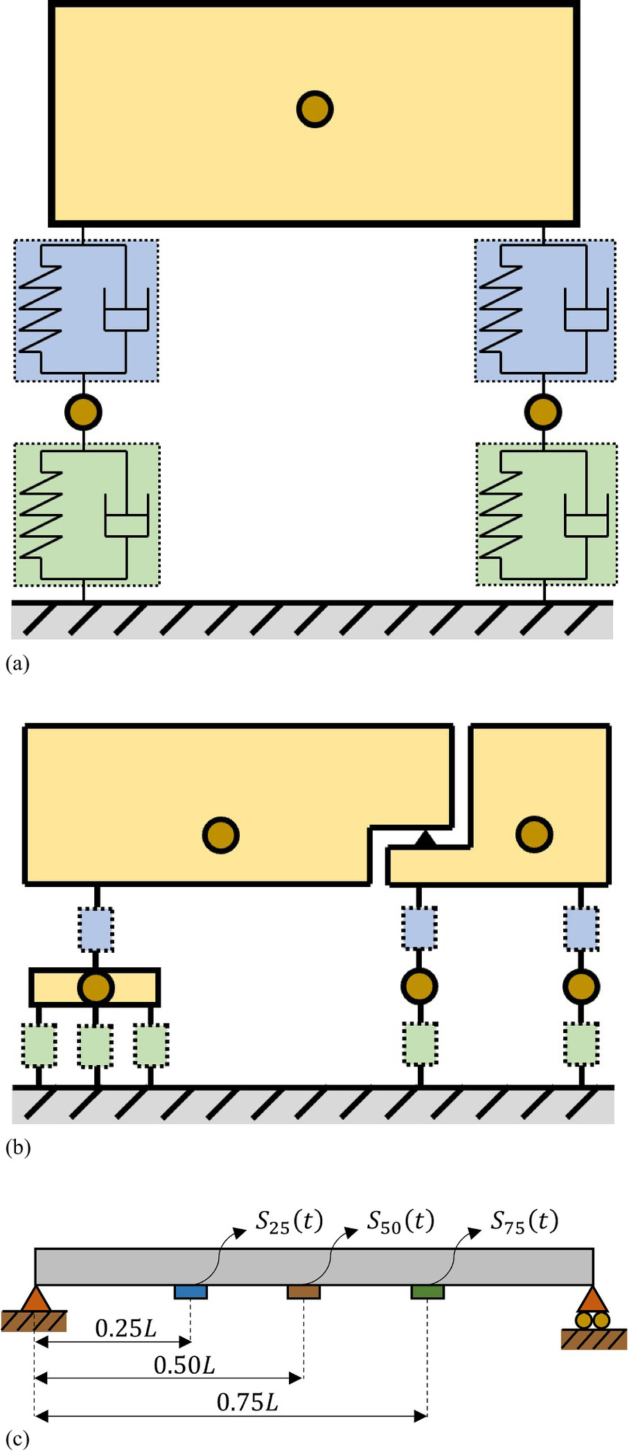
Table 1 shows the model properties used in this study to describe concrete bridges of different span lengths, which are based on the values reported by Li (2006) for an elastic modulus of 35 × 109 N/m2. On the other hand, the mechanical properties of the vehicles have been taken exactly as provided by Cantero and González (2015) for the two-axle vehicle and by OBrien et al. (2010) for the five-axle truck. In addition, the simulation includes road profile irregularities of Class A, according to the international standard ISO-8608 (ISO 1995). Because bridge responses under normal operational traffic conditions are expected to behave within the linear elastic range, which is an underlying assumption in BWIM installations, the linear numerical model used in this study is a valid proxy of the problem.
| Bridge span (m) | Mass per unit length (kg/m) | Second moment of area (m4) | Fundamental frequency (Hz) |
|---|---|---|---|
| 9 | 16,875 | 0.1139 | 9.4256 |
| 12 | 22,500 | 0.2700 | 7.0698 |
| 15 | 28,125 | 0.5273 | 5.6553 |
| 18 | 33,750 | 0.9113 | 4.7130 |
| 21 | 16,530 | 0.8722 | 4.8405 |
Convoluted Reciprocity
The quasi-static response of a bridge due to a passing vehicle can be calculated using the influence line. More precisely, the response at Location A is the convolution of the influence line at A by the loading function (Frøseth et al. 2017), as shown in the following equation:where P(t) = loading function, which is made of a series of impulse functions of magnitudes Pj, one for each axle j, that is time-shifted according to the axle distances and the speed of the vehicle v; and IA = influence line of the measured load effect at the Location A of the bridge.
(1)
Now, consider the influence line IB at another Location, B. The convolution of Eq. (1) by IB is
(2)
Using the definition in Eq. (1) and considering the commutative property of the convolution operator, Eq. (2) can be rewritten as follows:
(3)
This relation in Eq. (3) has been termed CR. The expression shows that the convolution of the response at Location A by the influence line at Location B is the same as the convolution of the response at B by the influence line at A. This is a simple yet powerful theoretical result that can be utilized for speed estimation. By definition, an influence line is described in the space domain. However, the influence lines, IA(x) and IB(x), can be transformed into the time domain by knowing (or assuming) the vehicle’s traversing speed v. The v value that satisfies Eq. (3) corresponds to the speed of the vehicle. This constitutes the basis of the proposed speed estimation method, which is illustrated in the “Speed Estimation Methods” section
Moreover, Eq. (3) can be extended to a more generic case. Multiplying it by the loading function PC(t), for a vehicle of known speed (called here calibration vehicle), gives the following equation:
(4)
Again, using the definition in Eq. (1), one can derive the following relationship:where SX,C(t) = measured response at location X due to the passage of the calibration vehicle. Eq. (5) indicates that the convoluted reciprocity relationship also exists between two Generic bridge locations A and B for responses for two independent vehicle crossing events.
(5)
Defining CRAB as the convolution of the response at A due to a vehicle by the response at B due to a second vehicle, Eq. (5) can be rewritten as follows:
(6)
This relationship [Eq. (6)] is valid for the responses of any two vehicles regardless of their axle configuration. Therefore, for the passage of a theoretical single-axle unit load vehicle and an unknown truck, the relationship gives Eq. (3) again.
Similar to previously with the influence lines, the signals for the (calibration) vehicle passage at known speed vC can be readily transformed into the space domain, SA,C(x) and SB,C(x). To estimate the speed of other vehicles, one can find the new value of v that satisfies Eq. (5). The speed estimation procedure based on calibration vehicle signals is called CRV here, whereas the procedure based on influence lines is referred to as CRI. Both approaches will be investigated separately because their results are somewhat different, and they have different practical implications.
Note that the aforementioned formulation was derived in terms of functions with continuous time (or space) as the argument. However, in practice, the signals and influence lines consist of arrays of values sampled at instances in time. Nevertheless, the aforementioned results are also valid for discrete representations of the quantities involved. Also, note that the previous derivation has considered only quasi-static effects. Real measured bridge responses due to passing vehicles also include dynamic components, which introduce perturbations and inaccuracies when using CR for speed estimation. Nevertheless, this simple idea provides a theoretical method to estimate vehicle speeds. Therefore, these ideas will be numerically and empirically validated in the following sections.
Speed Estimation Methods
This section presents an extended explanation of the main speed estimation strategies discussed in the “Introduction” section. All methods are evaluated for the same structural configuration and loading condition, which enables the direct comparison between the methods’ performances. In particular, the running example used in this section corresponds to the numerical simulation results for the simply supported 9-m-span bridge described in Table 1. The bridge is loaded by the two-axle vehicle shown in Fig. 1(a) traveling at a constant speed of 20 m/s (72 km/h). The simulation includes one realization of a Class A road profile and the coupling effect of the vehicle–bridge interaction, as described in the “Numerical Model” section. The bridge responses at three locations in the longitudinal direction [Fig. 1(c)] are the signals used for the speed estimation procedures in the following. When relevant, the methods are studied using the theoretical quasi-static or the total responses, where the latter responses also include the dynamic components. For the quasi-static case, ideally, any valid speed estimation method should be able to detect the speed without error.
It is acknowledged that the performances reported in the following are particular to the selected bridge and loading configuration. The performances are later evaluated for a larger range of configurations in the “Numerical Studies” section. Furthermore, note that no signal processing has been performed on the responses. This is to evaluate the intrinsic speed detection capability of each method without the possible improvement that any additional processing might provide.
Peak-to-Peak Method
A method to estimate the speed of a vehicle crossing event is by studying the time difference between peaks in the signals. One possibility is to use the times for maximum (or minimum) values of signals measured at separate locations. This idea applied to the quasi-static signals of the running example [Fig. 2(a)] gives a speed estimate of 180 m/s (800% error), which is not a valid result. However, this simple idea has worked for some ideal cases (OBrien and Žnidarič 2001) and has been used as an initial guess for more refined speed estimation methods.
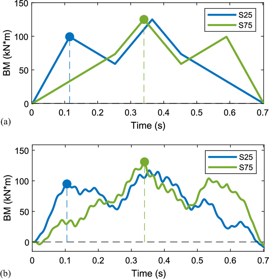
Alternatively, it is possible to work with the time differences between peaks that correspond to the same axle of the vehicle. For instance, this is illustrated for the peaks corresponding to the first axle in the quasi-static responses in Fig. 2(a). Knowing the distance between sensors, this idea provides a perfect speed estimation (0% error). However, when the signals include disturbances from the dynamic response, as shown in Fig. 2(b), the estimated speed is 19.15 m/s (−4.25% error). Therefore, this method might provide appropriate estimates, but it relies on the identification and matching of the peaks corresponding to vehicle axles.
Correlation
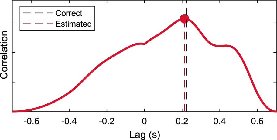
The most popular and established method to estimate speed is studying the correlation between two signals. The time lag that gives the highest correlation is used as an indication of the vehicle’s travel time from one sensor to the next. The underlying assumption for this method is that both signals match in shape when time-shifted. However, for BWIM systems, it is generally not possible to find two locations on the bridge that give the same signal for a passing vehicle. Nevertheless, it is often used because it provides appropriate speed estimates, particularly when the sensors capture local responses of the structure and the signals have very distinct peaks (Kalin et al. 2006). For the running example, the correlation between the quasi-static signals in Fig. 2(a) is shown in Fig. 3. The time lag corresponding to the maximum correlation is used to estimate the speed, which in this case is 21.18 m/s (5.88% error). Fig. 3 also shows the lag value to obtain the correct speed of the event. This example shows that the correlation method does not work perfectly, even in the case of quasi-static signals.
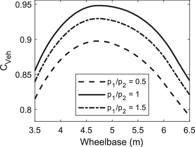
The discrepancies in speed estimates using the correlation method are well-known. Some correction strategies have been proposed to improve its accuracy and facilitate its use in a wider set of structural configurations. One such correction strategy relies on the definition of a calibration factor CVeh, which was reported in Liljencrantz et al. (2007) and has also been used in Zolghadri et al. (2016). This calibration factor is obtained by comparing the known speed of a passing vehicle to the result obtained with the correlation method. However, it can be shown that this calibration factor is specific for each vehicle since it depends on the number of axles, the spacing between them, and their relative load. Fig. 4 shows the calibration factor for a range of different axle spacings and axle weight distributions. The factor was calculated for the two-axle vehicle using ideal quasi-static responses of the bridge. Therefore, this correction strategy could be used only to estimate the speed of vehicles identical to the calibration vehicle, thus requiring different factors for different vehicles. This is not a practical strategy for road bridges due to the heterogeneity of the vehicles in traffic. However, this might be a feasible approach for railway bridges, where generally there exist only a limited number of types of locomotives. For completeness, the performance of the correlation method corrected with CVeh for the running example is reported in Table 2.
| Correction strategy | Quasi-static | Dynamic | ||
|---|---|---|---|---|
| Estimate (m/s) | Error (%) | Estimate (m/s) | Error (%) | |
| None | 21.18 | 5.88 | 21.43 | 7.14 |
| Calibration factor CVeh (Liljencrantz et al. 2007) | 20.00 | 0.00 | 20.24 | 1.19 |
| Qualified maxima (Kalin et al. 2006) | 20.00 | 0.00 | 19.15 | −4.26 |
Another correction strategy is suggested in Kalin et al. (2006) based on identifying a few qualified maxima (usually 2 or 3) in both signals. These maxima are points in the signals with certain requirements to ensure that they correspond to significant peaks and are not just simply local extremes. The correction strategy calculates the time differences for each pair of maxima and proceeds with the time difference that is closest to the time lag obtained by simple correlation. Indeed, this correction strategy improves the correlation method for quasi-static signals obtaining perfect speed estimation (0% error). When including dynamic components in the signals, the strategy identifies four points as qualified maxima, as shown in Fig. 5. These maxima occur at slightly different instances in time (compared to the quasi-static case), affecting the accuracy of the final speed estimation, as reported in Table 2.
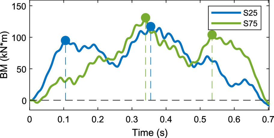
Table 2 summarizes the speed estimates for the running example using the correlation method and eventual correction strategy. For the ideal case (quasi-static response), the method works perfectly only when a correction strategy is applied. Even though the use of the calibration factor seems simple and reliable, it only works for the same vehicle configuration, rendering it impractical for road bridges. The correction based on qualified maxima is more general but requires peak identification in the signals, which is not necessarily always possible. On the other hand, when the dynamic responses are considered, the accuracies degrade even when including correction strategies. Inevitably, when introducing the disturbances in the ideal signals, the speed estimation errors deviate.
Signal Combination via PLA
Another possibility for speed estimation is combining multiple responses into signals that are better suited for the correlation method. This can be achieved with the PLA presented in Cantero (2021), which factors and adds the responses using a finite difference scheme. With this procedure, it is possible to obtain signals with the same shape at different locations along the beam when using equally separated sensors. The results are time-shifted symmetric signals that are ideal inputs for speed estimation by correlation.
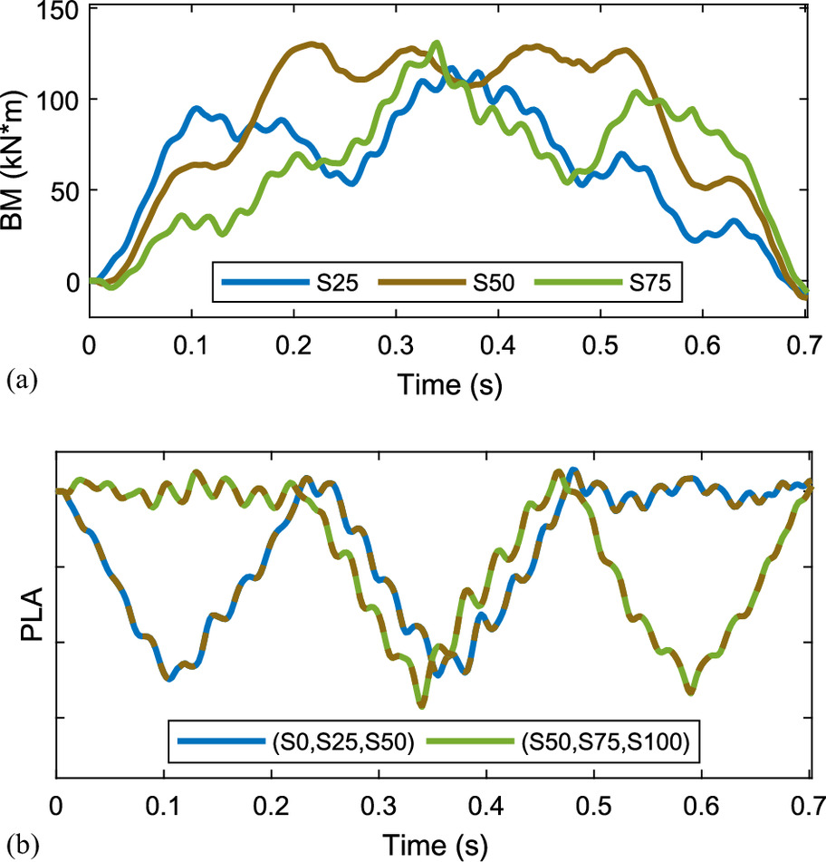
To illustrate this method on the running example, it is necessary to use additional sensor readings to those indicated in Fig. 1(c). As suggested in Cantero (2021), one possibility is to define virtual sensors located at the supports, which are known to give zero-valued signals. These five sensors (three real and two virtual) are equally spaced between each other and permit the fabrication of time-shifted versions of the same signal via PLA. The three nonzero signals for the running example are shown in Fig. 6(a), including dynamic effects. The first PLA signal can be obtained by combining the responses at 25% and 50% of the span together with the virtual sensor signal at the left support (0% of L). Similarly, the second PLA signal is the combination of S50 and S75 together with the virtual zero response at the right support (S100). The resulting PLA signals are shown in Fig. 6(b). As can be seen, even when including the dynamic effects, both PLA signals have remarkably similar shapes. The correlation method based on these PLA signals gives a speed estimate of 19.78 m/s (−1.10% error). Not shown here, but the same exercise using quasi-static signals renders a perfect speed estimation (0% error).
Convoluted Reciprocity
The theoretical relationship derived in the “Methods” section, called CR, can be used to obtain speed estimates based on influence lines or responses from calibration vehicles. In this section, the speed estimation is illustrated only using CRI, but a similar procedure and results are obtained using CRV.
The speed estimation method is described schematically in Fig. 7 for the case of the running example. First, the procedure requires information from two sensors, namely, their influence lines and the responses due to the passing vehicle of unknown speed. Then, the method rescales the influence lines assuming different speeds and evaluates the validity of the convoluted reciprocity equality [Eq. (6)]. For any given speed, the discrepancy between the right-hand side and the left-hand side of the equation is evaluated with the norm of their difference. The value that minimizes that difference is the estimated speed of the crossing vehicle.
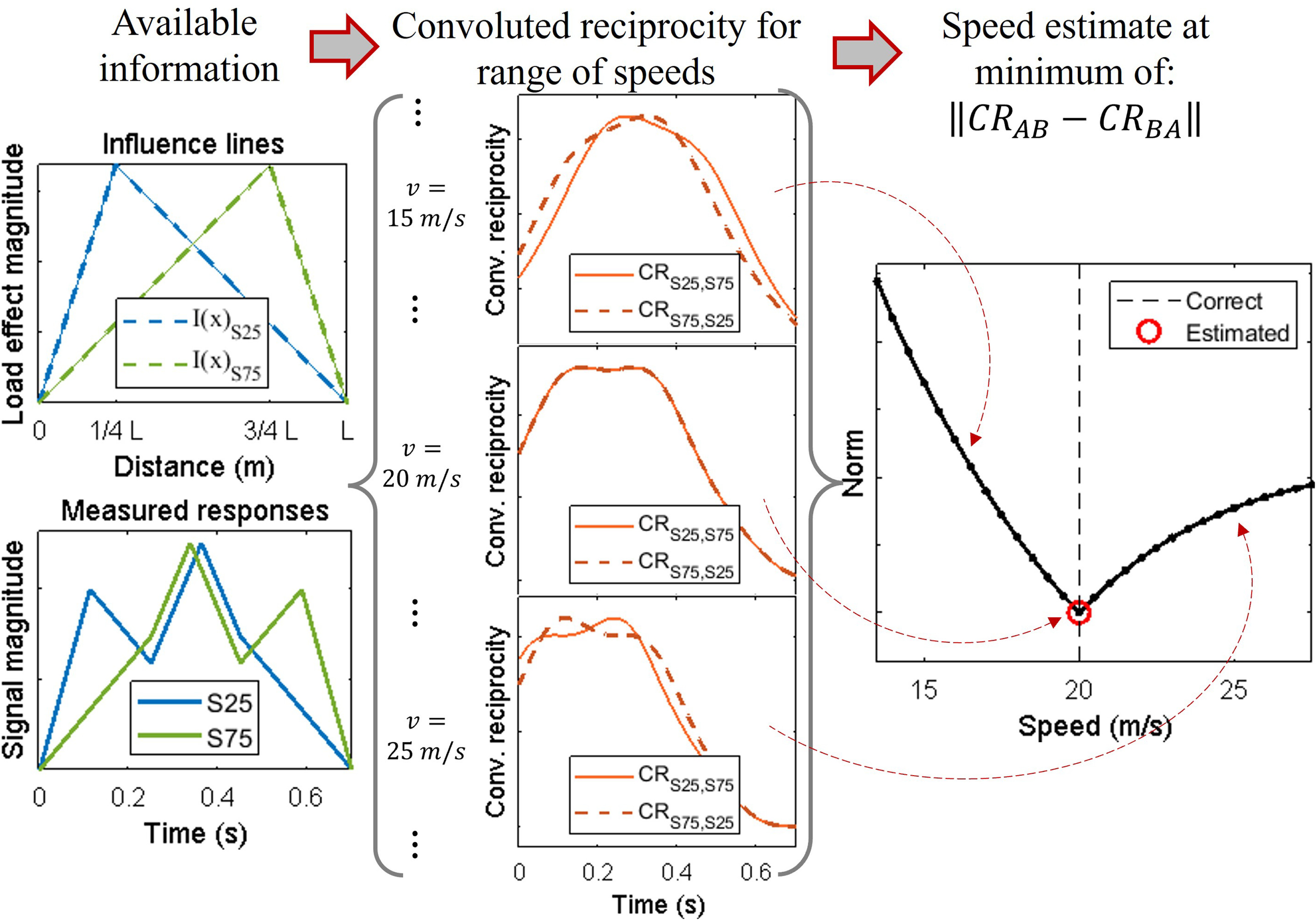
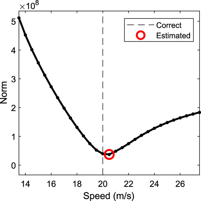
The illustrative example shown in Fig. 7 used the ideal quasi-static bridge responses and resulted in perfect speed estimation (20 m/s). However, when including the dynamic components of the bridge response in the signals, the convoluted reciprocity procedure provides a speed estimate of 20.41 m/s (2.06% error). For reference, Fig. 8 shows the norms of the convoluted reciprocity for the range of speeds considered, observing the small discrepancy due to the disturbances introduced by the dynamic components in the signals.
The procedure illustrated in Figs. 7 and 8 found the minimum norm from a parametric study on a range of speeds. However, this procedure can also be implemented as a numerical minimization problem. It was found that the objective function, namely the norm of the difference between convoluted reciprocities, is a convex function that features a single well-defined minimum. Adopting established optimization procedures is generally more computationally efficient and results in the same speed estimate (except for very small numerical discrepancies related to the discretization size and the adopted tolerances in the minimization procedure). In the remainder of this study, the vehicle speed via CR is obtained using MATLAB’s fminsearch command to find the minimum, which uses the simplex search method (MATLAB 2022).
Numerical Studies
This section presents numerical investigations based on Monte Carlo simulations to explore two aspects of the problem. The study in the following first searches for the best metric to use for the convoluted reciprocity procedure and then compares the performances of different speed estimation methods. The Monte Carlo simulation is performed on the five different bridge spans defined in Table 1, traversed by the two vehicle types shown in Fig. 1, namely, the two-axle vehicle and the five-axle articulated truck. The properties of the vehicles were randomly sampled following the variabilities defined in Cantero and González (2015) and OBrien et al. (2010) for the two-axle and five-axle vehicles, respectively, which resulted in crossing events with different geometries, axle loads, mass distributions, and suspension properties. Also, the speeds of the vehicles were randomly sampled from a uniform distribution for values in the range of 50–120 km/h (13.89–33.33 m/s). All these events were simulated traveling on a single random realization of a Class A road profile.
Best Metric
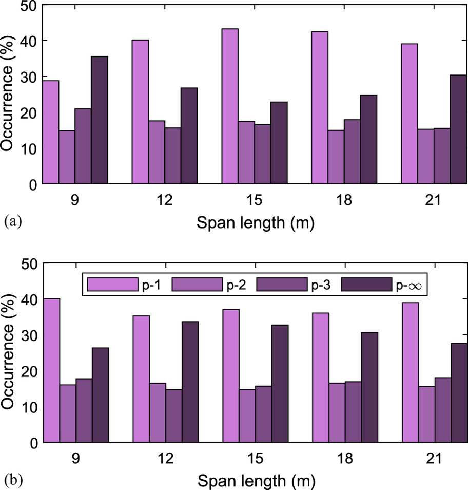
As described in Fig. 7, the speed estimation via the convoluted reciprocity used the norm as the metric to evaluate the similarity between both sides in Eq. (6). However, there exist different possibilities to define this norm. The generalized expression of p-norm (norm of order p) for a vector r is shown in Eq. (7), a definition that gives either the sum in absolute value (p = 1), the Euclidean norm (p = 2), or the maximum (p = ∞), among the possibilities:
(7)
A priori, it was not known what norm order would work best for the proposed speed estimation procedure. Therefore, this was evaluated numerically, studying the same problem for a selection of different norm orders. A Monte Carlo simulation with 4,000 events was used to identify what is the best metric to use as an indicator in the speed estimation procedure using the convoluted reciprocity. For each simulated event, the CR procedure was repeated for four different norms (1-norm, 2-norm, 3-norm, and ∞-norm). Fig. 9 shows the number of times (in relative terms) that each norm was identified as the best-performing metric. The results indicate that generally 1-norm seems to be the norm that most frequently best-identified speed. Therefore, the 1-norm was adopted as the default norm to evaluate the difference in the convoluted reciprocity expression.
Performance Comparison
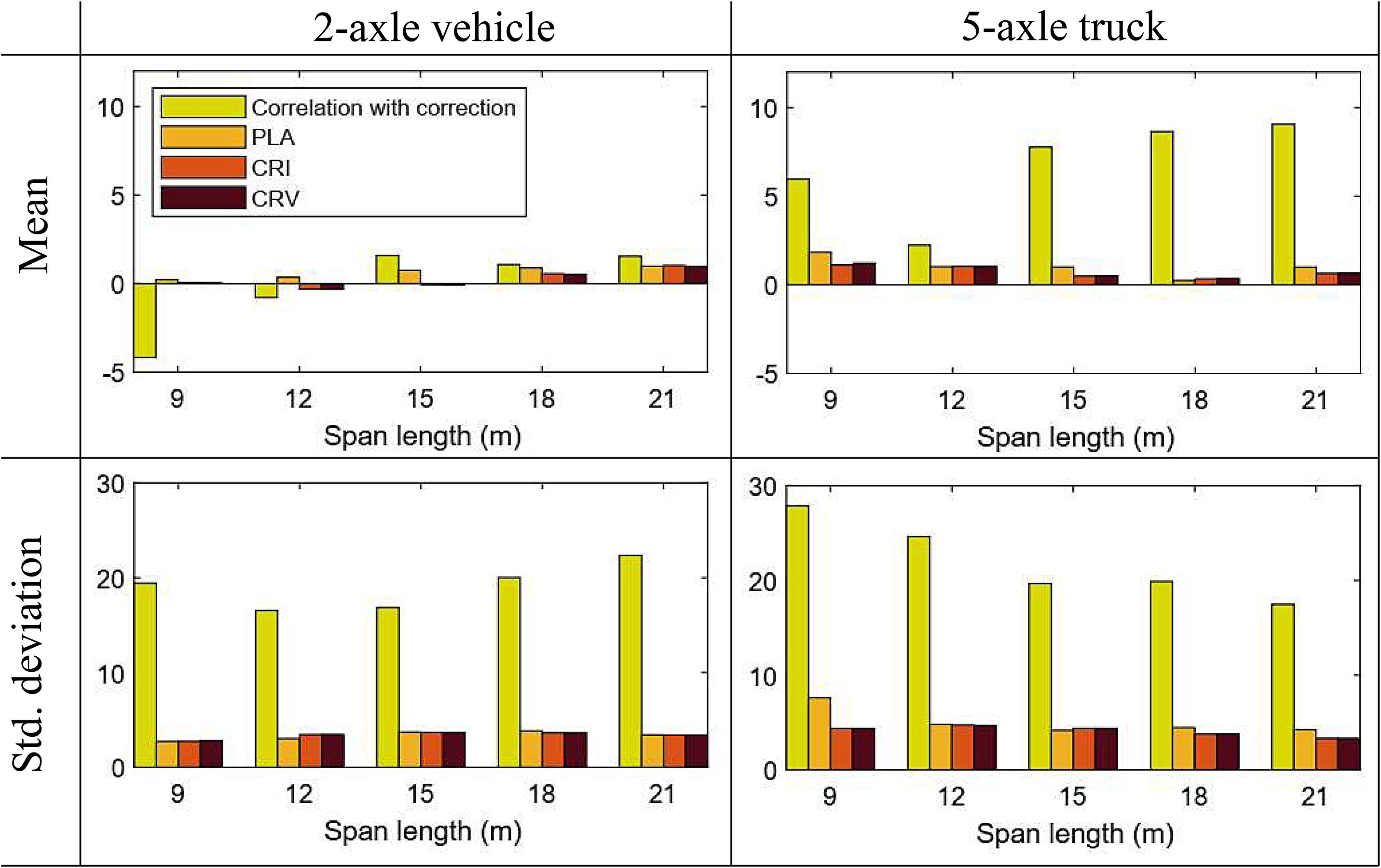
The “Speed Estimation Methods” section presents presents different speed estimation methods based on one single example in detail. To assess the actual performance of each of them, they must be tested under a range of structural configurations and loading scenarios. Therefore, a new Monte Carlo analysis was performed with 20,000 events to compare the performances of several speed estimation methods. In particular, the study evaluated the following methods:
1.
Correlation with correction: The correlation between signals from sensors at 25% and 75% of L, complemented by the correction strategy based on qualified maxima, as outlined in the “Correlation” section.
2.
PLA: Simple correlation (without any correction) using signals derived from combining two different sensor triads, as presented in the “Signal Combination via PLA” section.
3.
CRI: Speed estimation based on the convoluted reciprocity property using responses and influence lines at sensors 25% and 75% of L, as presented in the “Convoluted Reciprocity” section.
4.
CRV: Similar to the previous method but utilizing the quasi-static response of a two-axle calibration vehicle instead of influence lines.
Fig. 10 shows the mean error and corresponding standard deviation for each of the four methods, where the results are divided into bridge spans and vehicle types. In general, the results show that the correlation (with correction) does perform well enough for certain spans and vehicle types. However, its mean error can be significant (up to 9% error) in some cases. In addition, the correlation error displays large variability in performance, reflected in a large standard deviation. In comparison, the methods based on PLA and CR give consistently small mean errors and standard deviations. The results clearly indicate that PLA and CR approaches outperform the standard speed estimation method based on the correlation of two signals. To confirm these results and evaluate further the difference between methods, the study was continued under laboratory conditions with real measured signals and discussed in the next section.
Experimental Validation
Setup
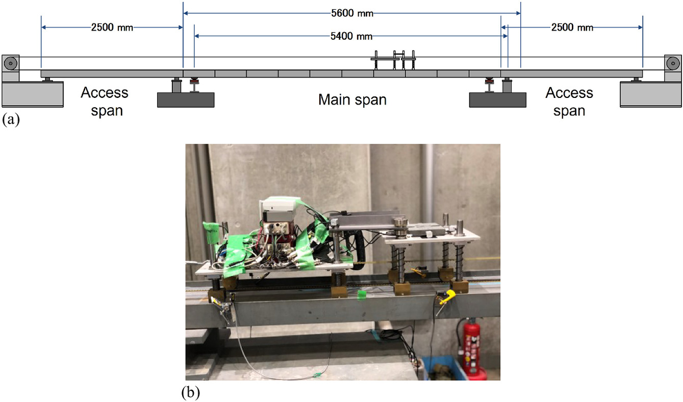
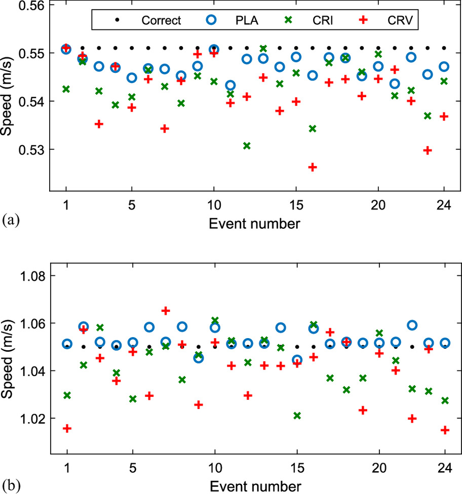
A vehicle crossing a bridge was experimentally reproduced in the laboratory using a scaled setup of a beam traversed by a model vehicle. Fig. 11 shows the four-axle model vehicle used in the experiment, which consisted of the main body and trailer with axle weights and spacing as provided in Table 3. The vehicle was moved across the access tracks and beam by a pulley system, which provided constant speed while crossing the beam. The vehicle was moved back and forth across the beam 12 times, which resulted in 24 crossing events. This loading sequence was performed for two different constant speeds, namely, at V1 = 0.551 and V2 = 1.048 m/s.
| Axle number | Weight (kg) | Axle spacing (mm) |
|---|---|---|
| 1 | 12.70 | 0 |
| 2 | 14.75 | 400 |
| 3 | 8.05 | 210 |
| 4 | 6.70 | 190 |
The beam, also shown in Fig. 11, was a 5.6-m-long steel beam in a simply supported configuration spanning 5.4 m. The properties of the beam are listed in Table 4. The 300-mm-wide Steel I-beam was positioned on the side, so the edges of the model bridge were the flanges, and the web constituted the deck on which the model vehicle was moving on. The vehicle was moving over steel rails with an imposed roughness corresponding to a Scaled class A ISO-8608 (ISO 1995) profile. The beam was instrumented with strain gauges located at 25% (= L/4), 50% (= L/2), and 75% (= 3L/4)of L, which resulted in signals S25, S50, and S75, respectively, adopting the same configuration and notation as in Fig. 1. The sampling frequency was 2,048 Hz using the NI9237 data acquisition system.
| Property | Value |
|---|---|
| Beam length | 5.6 m |
| Span length | 5.4 m |
| Elastic modulus | 210 × 109 N/m2 |
| Density | 7.8 × 10³ kg/m3 |
| Cross-sectional area | 7.04 × 10⁻³ m2 |
| Second moment of the area | 1.14 × 10⁻⁶ m4 |
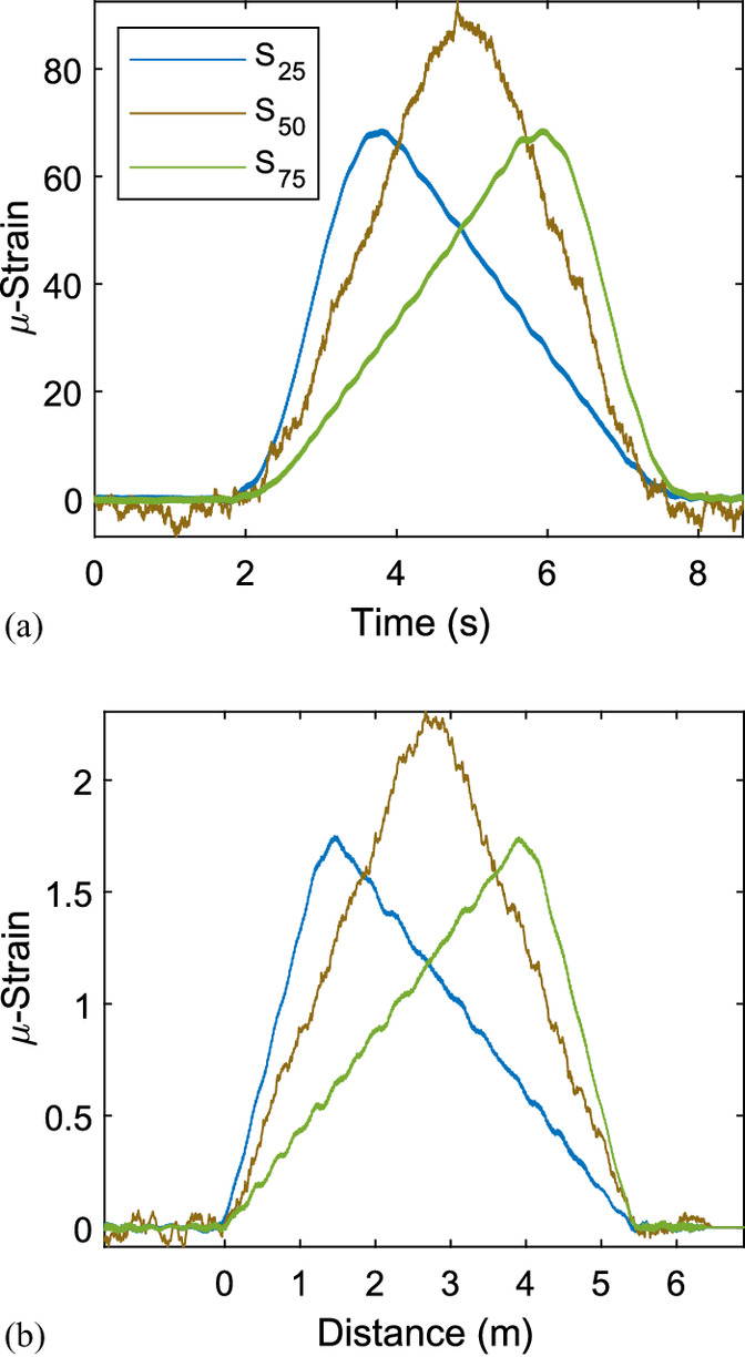
Fig. 12(a) shows a sample of the measured strain signals during a single-vehicle model passage traveling at V2 speed. These signals have been processed to remove noise with a zero-phase first-order Butterworth lowpass filter with a 1 Hz cutoff frequency. With the known information about the vehicle (Table 3) and traversing speed, the influence lines at each sensor location were obtained via the matrix method (OBrien et al. 2006). The final influence lines considered in this study [shown in Fig. 12(b)] are taken as the average result extracted from several vehicle passages.
Results
The three novel methods presented in this document were used to estimate vehicle speeds using the signals obtained from the laboratory experiments. First, the PLA method utilized the three recorded beam responses and assumed the existence of two virtual sensors at the supports to obtain signals of similar shape to subsequently estimate the speed via correlation. Also, both possibilities of the convoluted reciprocity approach were investigated separately. The CRI approach relied on the average influence lines presented in Fig. 12(b), whereas CRV employed the bridge responses for the first event with Speed V1. The estimated speeds for each method and event are shown in Fig. 13, where they can be compared against the correct value of the model vehicle. All three methods have certain variability in results but predict the speed with similar accuracy. There is no obvious trend or difference between methods.
To evaluate the speed estimation performance of each method, the results in Fig. 13 are summarized in statistical terms in Table 5. For completeness, this table also includes the results obtained using the correlation method with and without correction strategy. The results clearly show that for the novel speed estimation methods, the mean errors are one order of magnitude smaller than those based on correlation. As expected, the plain correlation method offered quite poor results. This was significantly improved when including the correction strategy based on qualified maxima. Nevertheless, on average, the estimated speeds showed more than 10% error and a significant dispersion in results. On the other hand, the results indicate that the PLA method offered the best performance, obtaining the smallest mean and standard deviation among all the methods. Then, the second-best method is CRI, closely followed by CRV, featuring average errors less than 2% and similar standard deviations.
| Method | Speed = 0.551 m/s | Speed = 1.048 m/s | ||
|---|---|---|---|---|
| Mean error (%) | Standard deviation (%) | Mean error (%) | Standard deviation (%) | |
| Correlation | 46.67 | 1.38 | 54.76 | 1.56 |
| Correlation + correction | 18.39 | 10.2 | 13.13 | 9.86 |
| PLA | −0.69 | 0.37 | 0.29 | 0.38 |
| CRI | −1.43 | 0.87 | −0.73 | 1.08 |
| CRV | −1.69 | 1.14 | −0.90 | 1.29 |
Discussion
This document presented and validated the idea of convoluted reciprocity. This theoretical finding provides a new way of solving the speed estimation problem. As seen in the “Methods” section, its derivation is based exclusively on the properties of the convolution operation. The result is independent of the properties, configuration, or boundary conditions of the structure. In that sense, the result is universal. The method can be used with any two sensor locations in the longitudinal direction.
Furthermore, it was shown that the CR relationship is valid for any type of vehicle. When that vehicle is a theoretical single axle of unit load, the relation is in terms of influence lines. However, the relationship is also valid for any vehicle of known speed. In theory, both approaches should give the same speed estimate. This is confirmed numerically and experimentally in this study. Any small discrepancies can be attributed to the effects of noise, dynamic components in the signals, and numerical rounding errors. One could argue that using CR in terms of the influence lines should give more accurate speed estimates since CRI is based on a calibrated response that is the result of multiple measurements. In fact, this was observed in the experimental analysis in Table 5, where the performance of the CRI is slightly better than the one based on the calibration vehicle. However, in practice, it might often be useful to estimate the speed based on the response of a single vehicle with a known speed, namely via CRV. That calibration vehicle could be forced to travel at the lowest speed allowed on that road to minimize the magnitude of the dynamic components in the bridge response, which would reduce the subsequent errors in speed estimates.
This document also showed the potential of using the PLA method for speed estimation. The combination of responses via a finite difference scheme provides signals that are more similar, which in turn are inputs that are better suited for the direct correlation method. In fact, the PLA method provided the overall best performance for the laboratory tests reported in Table 5. However, this method requires multiple sensor locations in the longitudinal direction, with equal distance between them. This might not always be a practical (or even possible) solution, and it might require more sensors than those found in standard BWIM installations. The PLA idea for speed estimation might be relevant in installations with a denser grid of sensing locations, for instance, when using fiber Bragg grating sensors.
Conclusion
This study focuses on the speed estimation problem for the most common BWIM installation, which utilizes strain measurements from the bridge at multiple locations. The literature review indicates that existing speed estimation methods have certain difficulties and limitations. This paper introduces a new concept, called CR, that provides a relationship between responses recorded at two separate locations for two independent crossing events. This simple yet powerful idea is used to propose a theoretically consistent method to determine the speed of passing vehicles. Two variations of the method are presented, namely, CRI based on the sensors’ influence lines and CRV based on the bridge response for a calibration vehicle. In addition, the study explores the use of PLA signals together with the correlation method as another possibility for speed estimation. The existing and novel methods are illustrated based on simulated bridge responses. Their performance is evaluated for a range of vehicle and bridge configurations, which showed that the newly proposed methods provide more accurate and robust speed estimates. To validate these results, this study performs laboratory tests of a scaled bridge traversed by a model vehicle. The analysis of the empirical data confirms the findings.
Therefore, this document presents, evaluates, and validates three new speed estimation methods: CRI, CRV, and PLA with correlation. All of them provide similar accuracies. Their practical implementation in BWIM systems depends on the sensor layout and calibration procedure. While CRI requires the knowledge of influence lines at two separate bridge locations, CRV works with the bridge response from a single vehicle of known speed. On the other hand, the PLA with correlation method needs an array of multiple sensors with equal spacing. In conclusion, these new methods provide accurate speed estimates for a range of practical BWIM implementations.
Data Availability Statement
All data, models, or codes that support the findings of this study are available from the corresponding author upon reasonable request.
References
Algohi, B., A. Mufti, and D. Thomson. 2018. “Detection of speed and axle configuration of moving vehicles using acoustic emission.” J. Civ. Struct. Health Monit. 8: 353–362. https://doi.org/10.1007/s13349-018-0281-8.
Bakht, B., and A. Mufti. 2015. Bridges. Cham, Switzerland: Springer.
Bao, T., S. K. Babanajad, T. Taylor, and F. Ansari. 2016. “Generalized method and monitoring technique for shear-strain-based bridge weigh-in-motion.” J. Bridge Eng. 21: 04015029. https://doi.org/10.1061/(ASCE)BE.1943-5592.0000782.
Cantero, D. 2021. “Moving point load approximation from bridge response signals and its application to bridge weigh-in-motion.” Eng. Struct. 233: 111931. https://doi.org/10.1016/j.engstruct.2021.111931.
Cantero, D. 2022. “VEqmon2d—Equations of motion generation tool of 2D vehicles with Matlab.” SoftwareX 19: 101103. https://doi.org/10.1016/j.softx.2022.101103.
Cantero, D., and A. González. 2015. “Bridge damage detection using weigh-in-motion technology.” J. Bridge Eng. 20 (5): 1–10. https://doi.org/10.1061/(ASCE)BE.1943-5592.0000674.
Chatterjee, P., E. OBrien, Y. Li, and A. González. 2006. “Wavelet domain analysis for identification of vehicle axles from bridge measurements.” Comput. Struct. 84: 1792–1801. https://doi.org/10.1016/j.compstruc.2006.04.013.
Chen, S.-Z., G. Wu, and D.-C. Feng. 2019. “Development of a bridge weigh-in-motion method considering the presence of multiple vehicles.” Eng. Struct. 191: 724–739. https://doi.org/10.1016/j.engstruct.2019.04.095.
Chen, S.-Z., G. Wu, D.-C. Feng, and L. Zhang. 2018. “Development of a bridge weigh-in-motion system based on long-gauge fiber bragg grating sensors.” J. Bridge Eng. 23 (9): 04018063. https://doi.org/10.1061/(ASCE)BE.1943-5592.0001283.
Debojyoti, P., and R. Koushik. 2023. “Application of bridge weigh-in-motion system in bridge health monitoring: A state-of-the-art review.” Struct. Health Monit. 22 (6): 4194–4232. https://doi.org/10.1177/14759217231154431.
Frøseth, G. T., A. Rønnquist, D. Cantero, and O. Øiseth. 2017. “Influence line extraction by deconvolution in the frequency domain.” Comput. Struct. 189: 31–30. https://doi.org/10.1016/j.compstruc.2017.04.014.
Hajializadeh, D., A. Žnidarič, J. Kalin, and E. J. Obrien. 2020. “Development and testing of a railway bridge weigh-in-motion system.” Appl. Sci. 10: 4708. https://doi.org/10.3390/app10144708.
He, W., L. Deng, H. Shi, C. S. Cai, and Y. Yu. 2017. “Novel virtual simply supported beam method for detecting the speed and axles of moving vehicles on bridges.” J. Bridge Eng. 22 (4): 04016141. https://doi.org/10.1061/(ASCE)BE.1943-5592.0001019.
Huseynov, F., D. Hester, E. J. Obrien, C. McGeown, C.-W. Kim, K. Chang, and V. Pakrashi. 2022. “Monitoring the condition of narrow bridges using data from rotation-based and strain-based bridge weigh-in-motion systems.” J. Bridge Eng. 27 (7): 1–13. https://doi.org/10.1061/(ASCE)BE.1943-5592.0001872.
ISO (International Organization for Standardization). 1995. Mechanical vibration—Road surface profiles—Reporting of measured data. ISO 8608. Geneva: ISO.
Jacob, B., E. J. OBrien, and S. Jehaes. 2002. COST 323 weigh-in-motion of road vehicles. Final Report. Paris: Laboratoire Central des Ponts et Chaussées.
Jian, X., Y. Xia, J. A. Lozano-Galant, and L. Sun. 2019. “Traffic sensing methodology combining influence line theory and computer vision techniques for girder bridges.” J. Sens. 2019: 3409525. https://doi.org/10.1155/2019/3409525.
Kalhori, H., M. M. Alamdari, X. Zhu, B. Samali, and S. Mustapha. 2017. “Non-intrusive schemes for speed and axle identification in bridge-weigh-in-motion systems.” Meas. Sci. Technol. 28: 025102. https://doi.org/10.1088/1361-6501/aa52ec.
Kalin, J., A. Žnidarič, and I. Lavrič. 2006. “Practical implementation of nothing-on-the-road bridge weigh-in-motion system.” In Proc., 9th Int. Symp. on Heavy Vehicle Weights and Dimensions. State College, PA: Pennsylvania State University.
Kim, S.-W., D.-W. Yun, D.-U. Park, S.-J. Chang, and J.-B. Park. 2022. “Vehicle load estimation using the reaction force of a vertical displacement sensor based on fiber bragg grating.” Sensors 22: 1572. https://doi.org/10.3390/s22041572.
Li, Y. 2006. “Factors afiecting the dynamic interaction of bridges and vehicle loads.” Ph.D. thesis, School of Architecture, Landscape and Civil Engineering, Univ. College Dublin.
Liljencrantz, A., and R. Karoumi. 2009. “Twim: A MATLAB toolbox for real-time evaluation and monitoring of traffic loads on railway bridges.” Struct. Infrastruct. Eng. 5: 407–417. https://doi.org/10.1080/15732470701478370.
Liljencrantz, A., R. Karoumi, and P. Olofsson. 2007. “Implementing bridge weigh-in-motion for railway traffic.” Comput. Struct. 85: 80–88. https://doi.org/10.1016/j.compstruc.2006.08.056.
Lydon, M., S. E. Taylor, D. Robinson, A. Mufti, and E. J. OBrien. 2016. “Recent developments in bridge weigh in motion (B-WIM).” J. Civ. Struct. Health Monit. 6: 69–81. https://doi.org/10.1007/s13349-015-0119-6.
MacLeod, E., and K. Arjomandi. 2022. “Enhanced bridge weigh-in-motion system using hybrid strain–acceleration sensor data.” J. Bridge Eng. 27 (9): 04022077. https://doi.org/10.1061/(ASCE)BE.1943-5592.0001924.
MATLAB. 2022. Version: 9.13.0 (R2022b). Natick, MA: MathWorks.
Moses, F. 1979. “Weigh-in-motion system using instrumented bridges.” Transp. Eng. J. 105 (3): 233–249.
Mustafa, S., H. Sekiya, S. Hirano, and C. Miki. 2021. “Iterative linear optimization method for bridge weigh-in-motion systems using accelerometers.” Struct. Infrastruct. Eng. 17 (9): 1245–1256. https://doi.org/10.1080/15732479.2020.1802490.
OBrien, E., M. A. Khan, D. P. McCrum, and A. Žnidarič. 2020. “Using statistical analysis of an acceleration-based bridge weigh-in-motion system for damage detection.” Appl. Sci. 10: 663. https://doi.org/10.3390/app10020663.
OBrien, E. J., D. Cantero, B. Enright, and A. González. 2010. “Characteristic Dynamic Increment for extreme traffic loading events on short and medium span highway bridges.” Eng. Struct. 32: 3827–3835. https://doi.org/10.1016/j.engstruct.2010.08.018.
OBrien, E. J., M. J. Quilligan, and R. Karoumi. 2006. “Calculating an influence line from direct measurements.” Proc. Inst. Civ. Eng. Bridge Eng. 159 (BE1): 31–34. https://doi.org/10.1680/bren.2006.159.1.31.
OBrien, E. J., and A. Žnidarič. 2001. Weighing-in-motion of axles and vehicles for Europe (WAVE) WP1.2: Bridge WIM systems. Bridge WIM systems (B-WIM) Alternative ref: WAVE (2001), Bridge WIM, Report of Work Package 1.2. Ljubljana, Slovenia: Zavod za gradbeništvo.
Ojio, T., C. H. Carey, E. J. Obrien, C. Doherty, and S. E. Taylor. 2016. “Contactless bridge weigh-in-motion.” J. Bridge Eng. 21 (7): 1–11. https://doi.org/10.1061/(ASCE)BE.1943-5592.0000776.
Sekiya, H., K. Kubota, and C. Miki. 2018. “Simplified portable bridge weigh-in-motion system using accelerometers.” J. Bridge Eng. 23 (1): 04017124. https://doi.org/10.1061/(ASCE)BE.1943-5592.0001174.
Stawska, S., J. Chmielewski, M. Bacharz, K. Bacharz, and N. Nowak. 2021. “Comparative accuracy analysis of truck weight measurement techniques.” Appl. Sci. 11: 745. https://doi.org/10.3390/app11020745.
van Loo, H., and A. Žnidarič. 2019. “Guide for users of weigh-in-motion.” In An introduction to weigh-in-motion. Radovljica, Slovenia: International Society of Weigh-in-Motion.
Yu, Y., C. S. Cai, and L. Deng. 2016. “State-of-the-art review on bridge weigh-in-motion technology.” Adv. Struct. Eng. 19 (9): 1514–1530. https://doi.org/10.1177/1369433216655922.
Zhou, Y., Y. Pei, S. Zhou, Y. Zhao, J. Hu, and W. Yi. 2021. “Novel methodology for identifying the weight of moving vehicles on bridges using structural response pattern extraction and deep learning algorithms.” Measurement 168: 108384. https://doi.org/10.1016/j.measurement.2020.108384.
Žnidarič, A., J. Kalin, and M. Kreslin. 2018. “Improved accuracy and robustness of bridge weigh-in-motion systems.” Struct. Infrastruct. Eng. 14: 412–424. https://doi.org/10.1080/15732479.2017.1406958.
Zolghadri, N., M. W. Halling, N. Johnson, and P. J. Barr. 2016. “Field verification of simplified bridge weigh-in-motion techniques.” J. Bridge Eng. 21: 04016063. https://doi.org/10.1061/(ASCE)BE.1943-5592.0000930.
Information & Authors
Information
Published In

Journal of Bridge Engineering
Volume 29 • Issue 2 • February 2024
Copyright
This work is made available under the terms of the Creative Commons Attribution 4.0 International license, https://creativecommons.org/licenses/by/4.0/.
History
Received: Apr 12, 2023
Accepted: Oct 6, 2023
Published online: Dec 5, 2023
Published in print: Feb 1, 2024
Discussion open until: May 5, 2024
Authors
Metrics & Citations
Metrics
Citations
Download citation
If you have the appropriate software installed, you can download article citation data to the citation manager of your choice. Simply select your manager software from the list below and click Download.