Particle Swarm Optimization of Interface Constitutive Model Parameters for Embedded Beam Formulations
Publication: International Journal of Geomechanics
Volume 24, Issue 11
Abstract
The numerical simulation of boundary value problems involving a high number of pile-type structures, such as pile foundation systems of high-rise buildings, represents a standard task in computational geotechnics. Due to their ability to simplify the underlying pile modeling process and decrease the simulation runtime embedded beam formulations (EBFs) have attracted widespread interest from the geotechnical community. State-of-the art EBFs are typically equipped with nonlinear interface constitutive models to capture the soil–structure interaction behavior with reasonable accuracy. However, reliable information concerning the calibration of related parameters is limited, which decreases the confidence in the results obtained with EBFs. The present work addresses this research aspect for the first time, along with a theoretical discussion of inherent simplifications in the numerical description of the soil–structure contact associated with EBFs. The significance of selecting adequate embedded interface constitutive model parameters to ensure EBF predictions with high credibility is demonstrated by means of parametric studies. This has motivated the development of an automatic calibration software, leveraged by particle swarm optimization, that provides guidance in selecting suitable values. The effectiveness of the calibration software is confirmed by back-calculation of different pile problems with default and calibrated parameter sets. Likewise, the results provide insight into crucial factors driving the calibration framework, with a view to increasing its potential for take-up in engineering practice. Potential lines of research in the context of the automatic calibration software are explored throughout this work and may serve as valuable reference in future research.
Practical Applications
The design of geotechnical problems involving a high number of pile-type structures, such as pile foundation systems of high-rise buildings or wind turbines, is routinely assisted by finite-element analyses. The computational expense of these simulations is significantly influenced by the pile modeling technique. Due to their exceptional ability to simplify the underlying modeling process and reduce the runtime to an acceptable limit, embedded beam formulations have therefore attracted widespread interest for geotechnical design tasks. As with all soil–structure interaction problems, it is essential in embedded beam formulations to accurately describe the interface behavior between the soil and the structure. This work presents the first attempt to highlight the relevance of this concern and visually describes relevant limitations resulting from an inadequate selection of interface constitutive model parameters. This observation has motivated the development of an automatic calibration software to increase the confidence in the parameter selection. The high potential of this software to increase the credibility of numerical predictions obtained with embedded beam formulations is demonstrated based on pile problems with different soil stratification layers, pile geometries, and pile arrangements. In all cases considered, the results confirm that the numerical fidelity could be significantly increased by employing calibrated parameter sets.
Introduction
The numerical simulation of geotechnical problems involving a high number of rather one-dimensional (1D) slender structures with high length-to-diameter ratios represents a challenging task. Pile-supported deep foundations (Ninić et al. 2014; Scarfone et al. 2020), micropile reinforcement systems (Esmaeili et al. 2013; Abbas et al. 2021), and soil-nailed walls (Lo 2014; Granitzer et al. 2021) are a case in point, in which simulation engineers seek to strike a balance between adequate accuracy of numerical results and reasonable computational expense. In these works, embedded beam formulations (EBFs) have become a main workhorse for modeling slender structures in an explicit manner, particularly due to their exceptional ability to reduce the simulation runtime to an acceptable limit (Granitzer et al. 2024). The widespread interest of the computational geotechnics community in EBFs is additionally manifested by their large diffusion in commercial finite-element (FE) codes, such as Diana 3D, ZSoil 3D, RS3, FLAC 3D, and PLAXIS 3D (Granitzer and Tschuchnigg 2021).
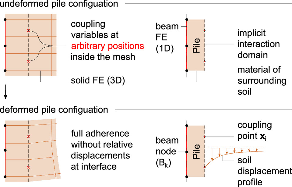
From a numerical point of view, EBFs represent a special group of overlapping domain decomposition methods (Cai 2003), which constitute a general framework for improved scalability and efficiency in the solution of large-scale boundary value problems (BVPs). As a key characteristic of this model class, EBFs describe the soil–structure interaction (SSI) behavior at an implicit interaction domain (Fig. 1). This requires the incorporation of mixed-dimensional coupling schemes, established between the 1D beam FE and the surrounding three-dimensional (3D) solid FEs, which track the coupling variables at arbitrary positions inside the mesh. Essentially, this feature allows for lifting computationally expensive meshing constraints associated with classical slender structure modeling techniques (Goudarzi and Simone 2019). The readers should notice, however, that the numerical description of the SSI behavior at the implicit interaction domain of EBFs is traditionally driven by desirable numerical properties or simplifying assumptions, rather than by profound calibration procedures, for example:
•
Full adherence between the embedded slender structure and surrounding soil, such that all modes of relative motion between the contacting bodies at the interaction domain are suppressed (Turello et al. 2016) (Fig. 1).
•
Reproduction of the initial slope in the load–settlement curves of vertically loaded single piles, such that the mechanical response is independent of interface elements (Tschuchnigg and Schweiger 2015).
•
Well-posedness of the tangent stiffness matrix to prevent the potential occurrence of unwanted contact locking phenomena leading to an unrealistically stiff response (Steinbrecher et al. 2020).
•
Suppression of discontinuities evolving at the implicit interaction domain in the solid mesh, as well as numerical oscillations in both the computed slip profiles (Goudarzi and Simone 2019) and mobilized skin traction distributions (Granitzer and Tschuchnigg 2023b).
While the numerical credibility of EBFs implemented based on one or more of these modeling assumptions may be suitable for certain boundary conditions (Engin et al. 2008; Engin and Brinkgreve 2009; Oliveria and Wong 2011; Sheil and McCabe 2012; Tradigo et al. 2016; Banerjee et al. 2020), it is worth noting that the results of various publications (Al-abboodi and Sabbagh 2019; Abo-Youssef et al. 2021; Granitzer and Tschuchnigg 2021; Granitzer and Felic 2022) indicate that their applicability for modeling slender structures is constrained. This discrepancy is not surprising because it can be explained by the simplifying factors in the numerical description of the SSI behavior, which are not necessarily suitable for the problem at hand.
Although a deep theoretical discussion of contact nonlinearities controlling the physical SSI behavior in the interface zone of slender structures is beyond the scope of the present paper, it should be noted that the underlying mechanism is influenced by numerous factors, including particle characteristics (Uesugi and Kishida 1986), soil properties (Kavitha et al. 2016), confinement conditions (DeJong and Westgate 2009), and structural surface characteristics (Potyondy 1961). Considering this complex nature of the SSI mechanism, in combination with the simplified rationales underlying the numerical description of the SSI behavior at the implicit interaction domain, it appears almost logical that numerical analyses addressing the mechanical behavior at critical locations in the near field of EBF interfaces should be regarded as first-order estimates and therefore used with care (Tschuchnigg and Schweiger 2015); for example, this may concern detailed numerical analyses of isolated piles with particular focus on pile installation effects, such as soil plugging (Henke and Grabe 2008) and excess pore-water pressure concentrations caused by cyclic loading (Staubach et al. 2020), fully coupled hydromechanical analyses of seepage flow around slender structures (Chen et al. 2022), or the influence of volumetric behavior at the soil–pile interface on the mechanical response of piles (Peng et al. 2014; Engin et al. 2015). Nevertheless, the majority of numerical simulations involving numerous slender structures are traditionally restricted to global response analyses, without transient water flow, and carried out under the premise that installation effects have an insignificant impact on their mechanical response (de Gennaro et al. 2008; Granitzer and Tschuchnigg 2021). In the realm of the so-called wished-in-place conditions, advanced EBFs that are equipped with nonlinear interface constitutive models have the potential to realistically capture the SSI behavior of slender structures, while preserving relative merits in terms of simulation runtime; relevant nonlinear features include the stress-dependent formulation of interface constitutive models (Tschuchnigg 2012; Turello et al. 2017) and the incorporation of frictional failure along the shaft (Sadek and Shahrour 2004; Tschuchnigg and Schweiger 2015).
Essentially, the use of nonlinear interface constitutive models in EBFs raises the obvious question as to what interface constitutive model parameters (ICMPs) should be selected to resemble the desired mechanical response with sufficient accuracy. In this context, it is important to notice that the choice of adequate values for ICMPs, which is the core of this work, represents a nontrivial task that renders an optimization problem similar to the calibration of soil models (Mendez et al. 2021; Machaček et al. 2022; Kadlíček et al. 2022). The salient difference concerns the optimization domain, which has to be expanded from stress point observations, where emphasis is usually placed on the influence of soil material parameters on the constitutive response in soil element tests (e.g., triaxial or oedometric tests), to full-scale BVPs in the discrete form comprising EBFs and the surrounding soil material. This aspect renders the calibration of ICMPs challenging since it increases the number of unknowns in the numerical integration algorithm and requires the design of efficient calibration procedures to restrain the computational effort to stay beyond practical limits. Moreover, the optimal solution to the calibration problem may be prone to the adopted mesh topology, particularly because the exact solution to BVPs involving EBFs may contain determinant singularities in the sought field variables. Interested readers may refer to Steinbrecher et al. (2020), where this aspect is theoretically discussed.
From the previous discussion, it becomes apparent that the influence of ICMPs on the numerical fidelity of EBFs remains unclear to a large extent. Needless to say, spurious predictions resulting from an inadequate selection of ICMPs may have adverse consequences in the interpretation of numerical results. This distinct lack of research is additionally highlighted in Remark 3.4 of a recent publication (Granitzer et al. 2024), which has further motivated this research. In this context, and to the authors’ best knowledge, the present work represents the first attempt to investigate the influence of ICMPs on the numerical response of geotechnical structures modeled by means of EBFs and to provide an automatic framework for their calibration. For this purpose, the remainder of this paper is organized as follows: At first, relevant implementational aspects of state-of-the-art EBFs are reconsidered, with particular emphasis on differences in their interaction domain geometry and interface constitutive model, as both aspects play an important role in the selection of suitable ICMPs. Next, we introduce an automatic calibration framework (ACF), including the definition of the objective function, optimization method, similarity measure, and search space constraints. On this basis, the capabilities of the calibration software are studied considering three well-documented pile problems. Finally, we draw the main conclusions of this work and highlight areas for further research.
Subsequently, the mathematical details are provided in symbolic notation where scalars are denoted by means of Greek and italic letters, for example, and . Lowercase bold letters are used to denote vectors, for example, .
Background
EBFs used in the field of computational geotechnics are principally classified according to their interaction domain geometry (Granitzer et al. 2024). This implementational feature deserves particular attention because it considerably governs the ability of an EBF to achieve mesh-independent results (Turello et al. 2016; Granitzer and Tschuchnigg 2021; Truty 2023). Consequently, it can be inferred that the potential of calibration procedures to determine adequate ICMPs, which remain valid across various mesh discretizations, depends on the interaction domain geometry employed with the EBF. For this purpose, the calibration framework developed in this work is tested on two EBFs with different interaction domain geometries, namely, the embedded beam with a line interface proposed by Tschuchnigg and Schweiger (2015) and the embedded beam with an interaction surface first applied by Smulders et al. (2019) and subsequently extended by Granitzer et al. (2024). For the sake of clarity, these are abbreviated as EB-L* and EB-I*, respectively. In this section, we shed light on the embedding method of both EBFs, with particular focus on the physical interpretation of their ICMPs. These theoretical considerations form the basis for the automatic calibration framework developed in this work.
Embedded Beam Formulations
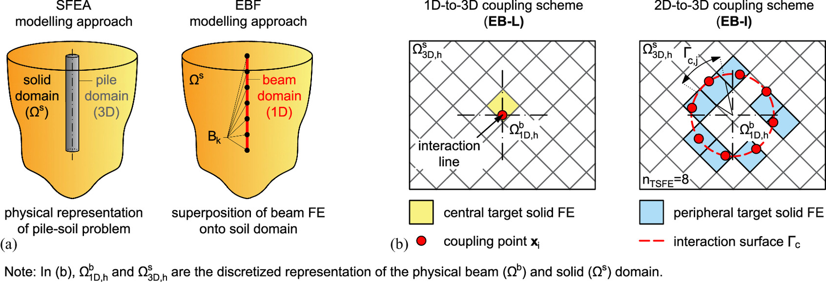
Over a period of more than four decades, the development of EBFs has been motivated by the increasing demand for computationally efficient slender structure modeling techniques. Early work has been executed in the field of structural concrete, where EBFs have been found eligible for the modeling of reinforcing agents (Phillips and Zienkiewicz 1976; Chang et al. 1987). With regard to the field of computational geotechnics, EBFs have been first employed by Sadek and Shahrour (2004) for the analysis of micropiles. In comparison with the traditional standard FE approach (SFEA) shown in Fig. 2(a), where piles are explicitly discretized by means of 3D solid FEs and interface elements to account for SSI effects, EBFs offer several desirable features of practical relevance, listed as follows:
•
A more flexible mesh generation procedure with independent discretization of the 3D solid domain ( ) and the 1D beam domain ( ) representing the slender structure (Sadek and Shahrour 2004) (Fig. 1).
•
Simplified evaluation of stress resultants (e.g., bending moment and normal force) without posterior integration of stress field quantities (Granitzer and Felic 2022).
•
A reduced number of unknowns in the discrete system of equations, resulting in a significantly improved simulation runtime efficiency (Granitzer et al. 2024).
These relative merits render EBFs particularly suitable for iterative design procedures, such as described in Di Prisco et al. (2020) and Jürgens et al. (2022), which greatly benefit from the arbitrary positioning of beam nodes inside , as opposed to the SFEA where mesh conformity constraints persist (Steinbrecher et al. 2020).
In view of the available methods for embedding in , EBFs can be classified as embedded beam FEs with interaction line (EB-Ls) and embedded beam FEs with interaction surface (EB-Is) (Granitzer et al. 2024). In the pertinent literature, these approaches are also referred to as local and nonlocal embedding methods (Truty 2023), both of which are addressed in this work. Fig. 2(b) visually explains the key difference between both embedding methods based on a single-pile problem: EBFs classified as EB-Ls are equipped with a multipoint line-to-volume (1D-to-3D) coupling scheme, i.e., contact conditions between the beam nodes ( ) and the surrounding target solid FE nodes ( ) are formally described at multiple coupling points placed along the centerline of (Tschuchnigg and Schweiger 2015). Assuming full adherence between and (Fig. 1) means that the motion of is fully controlled by the displacements of the central target 3D solid FE (TSFE) in which it is embedded [Fig. 2(b)]. This can be formally written as (Sadek and Shahrour 2004)where and are the displacement vectors with colocal origin . and are the element function and displacement vector, respectively, related to the th node of the central TSFE that is equipped with solid nodes. is the local position vector of described in the local coordinate system of the reference element associated with the central TSFE. To determine , it is required to solve the following system of equations for all ’s:where position vector of the th TSFE node.
(1)
(2)
Recent research has paved the way to EB-I models that allow for capturing the coupling between and in a more general manner compared to EB-L methods (Turello et al. 2016; Smulders et al. 2019; Granitzer and Tschuchnigg 2021, 2023c). The basic idea of the underlying embedding method is to dispatch the coupling contributions onto a larger set of [cf. Truty (2023)]. Instead of employing geometrically reduced 1D-to-3D configurations, as incorporated by EB-Ls, EB-Is are equipped with a surface-to-volume (2D-to-3D) coupling scheme. In this way, the numerical SSI behavior is defined at multiple peripheral ’s spread along the physical soil–structure interface [Fig. 2(b)]. Depending on the mesh topology, the coupling points are therefore enclosed by nonidentical peripheral TSFEs. As a consequence, the kinematical constraints have to be modified and incorporated in nonlocal form:where global weight that accounts for the area fraction of the peripheral interaction surface segment [Fig. 2(b)]; and local position vector of described in the local coordinate system of the respective peripheral TSFE. From Eq. (3), it becomes obvious that the motion of is coupled to the nodal displacements of multiple peripheral TSFEs, as opposed to EB-Ls. Favorable effects of this enhanced 2D-to-3D coupling scheme are highlighted in a number of publications (Turello et al. 2016; Smulders et al. 2019; Granitzer and Tschuchnigg 2021; Granitzer and Felic 2022; Granitzer and Tschuchnigg 2023c). A particularly relevant advantage of EB-Is is the reduced mesh size sensitivity. This can be explained by the distributed mobilization of coupling forces that reduce the influence of singularities on the numerical predictions. As will be demonstrated in this paper, this aspect has an important implication on the calibration of ICMPs.
(3)
For the sake of brevity, this subsection has focused on a comparative discussion of EB-Is and EB-Ls to facilitate understanding of the interface constitutive models, as well as the comparative study discussed later in this work. For a more comprehensive description of implementational details, including a mathematical description of alternative methods for the treatment of contact constraints between and , interested readers can refer to Turello et al. (2018), Steinbrecher et al. (2022b), and Granitzer et al. (2024).
Numerical Description of Soil–Structure Contact
The soil–structure interface behavior of vertically loaded piles is characterized by displacement gradients that develop within a concentrated shear zone in the soil (Hu and Pu 2004; DeJong et al. 2006; Martinez et al. 2015). As shown in Fig. 3(a), pile displacements may thus be regarded as the sum of soil displacements (i.e., developing in the soil surrounding the local zone of shearing) and local shear displacements (DeJong and Westgate 2009) [compare Lee and Xiao (2001)]. The latter are confined by particle size-dependent shear zones, which have a shear zone thickness of approximately , where is the mean grain size (Muir Wood 2002; Staubach et al. 2022). In this regard, it should be pointed out that this localized phenomenon forms within a zone spanning one FE in width (Ni et al. 2018b). To capture the shear localization with the finite-element method in a discrete manner, it is therefore required to use very thin solid FEs to represent the soil immediately adjacent to the interface (Potts and Zdravkovic 2001). Particularly in large-scale BVPs involving numerous piles (Tafili et al. 2023), however, this modeling technique leads to simulation runtimes that must be regarded as unbearable for most practical purposes (Ninić et al. 2014).
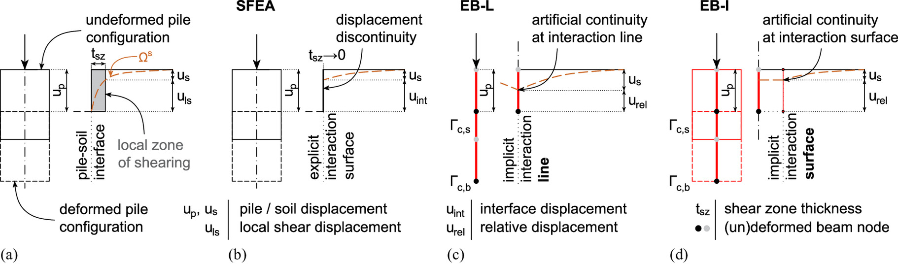
Alternatively, zero-thickness interface FEs could be used to overcome this problem (Ninić et al. 2014), as deployed in the SFEA [Fig. 3(b)]. This modeling approach aggregates the interface displacements , corresponding to , such that they become manifest in a boundary discontinuity where . Particular advantages of this modeling approach are the ability to vary the interface constitutive behavior (e.g., the maximum friction angle) and the reduction of solid FEs with high mesh density close to the soil–structure interface leading to an improved simulation runtime. For this purpose, the SFEA is commonly used as a numerical benchmark solution to assess the credibility of novel EBFs; for example, see Engin et al. (2007), Tschuchnigg and Schweiger (2015), Turello et al. (2016), Granitzer and Tschuchnigg (2023a), and Truty (2023).
Contrary to the SFEA, EBFs represent the pile domain by means of dimensionally reduced 1D beam FEs and impose the coupling constraints between and in a pointwise manner at the implicit interaction domain (Fig. 2). In this regard, the readers should notice that there is no explicit geometry object in the 3D solid mesh to match the pile domain (Granitzer et al. 2024). While this pile modeling strategy proves beneficial in terms of modeling and computational efforts, it is unable to capture the discontinuities in the solid mesh. This limitation, also referred to as artificial continuity (Goudarzi and Simone 2019), applies for both embedding methods described in Figs. 3(c and d) and has important implications with respect to the numerical description of the soil–structure interface behavior (Granitzer and Tschuchnigg 2023c):
•
The accurate representation of local field variables (e.g., stresses and strains) within the local zone of shearing lies beyond the capabilities of EBFs.
•
Relative displacements developing at the interaction domain between and have a limited physical meaning since they are not manifested in the solid domain, as opposed to the SFEA where can be numerically measured [Figs. 3(b–d)]. As a consequence, the representation of is, to some extent, restricted to the kinematic response of . This concern applies for both embedding methods, albeit being considerably improved with the 2D-to-3D embedding method associated with EB-Is.
These theoretical considerations imply that the ICMPs of EBFs should be calibrated considering the global pile response (e.g., using load–settlement curves obtained from static pile load tests), instead of comparisons between experimentally measured and simulated relationships in stress–strain spaces, as typically carried out for the calibration of soil constitutive model parameters.
Nonlinear Interface Constitutive Model
Both EBFs considered in this work (EB-L* and EB-I*) are equipped with advanced interface constitutive models, built on the principle of displacement coupling (Steinbrecher et al. 2022a). Contrary to simplified EBFs that consider full adherence between and , as shown in Fig. 1, they allow for capturing nonlinear effects of practical relevance, e.g., gap formation under tensile normal stresses and shear failure at the interaction domain. To realistically describe the mobilization of skin tractions along the shaft, the energy-conjugated pairs of relative displacements and skin tractions in the axial direction are related in a pointwise manner using empirical relationships. These are specified on the basis of extensive studies and have been found suitable for numerous problems of practical relevance (Tschuchnigg 2012). With regard to the EB-L*, the constitutive equations read (Tschuchnigg and Schweiger 2015)A similar approach has been adopted for the EB-I*, with the difference that the relations defined in Eq. (4) are additionally divided by the circumference and base area of the virtual beam geometry (Granitzer et al. 2024):In Eqs. (4) and (5), is the virtual beam radius and is the average shear stiffness of the TSFEs belonging to the set of located at the shaft ( ) and base ( ) interaction domain. It is important to note that the scalar-valued embedded interface stiffness multipliers and have been incorporated for calibration purposes. To the best of the authors’ knowledge, however, it is not publicly reported how these parameters affect the mechanical response of the EB-L* and EB-I*, respectively, and how the quality of numerical predictions can be improved by employing calibration procedures to select optimal values.
(4)
(5)
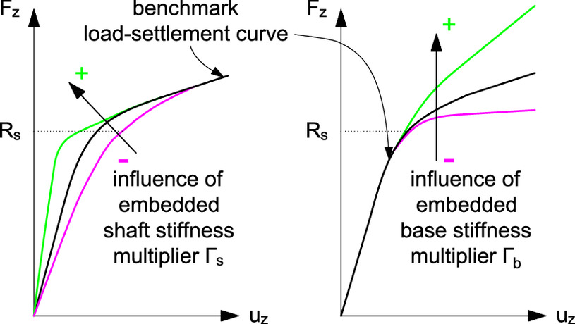
To shed light on these unsolved questions, Fig. 4 for the first provides insight into the influence of the embedded interface stiffness multipliers on the global response of an isolated pile modeled by means of the EB-L* and EB-I*. While the ultimate shaft resistance , obeying to a Coulomb-type failure criterion (Tschuchnigg and Schweiger 2015; Smulders et al. 2019), remains relatively unaffected, and considerably influence the predicted pile resistance mobilization rates along the full range of loading. From this point of view, it appears imperative to select appropriate values for these ICMPs, mathematically expressed by the parameter vector , to approximate the benchmark pile response with high accuracy.
Provided that the ultimate shaft capacity is reasonably captured by the pile model, the aforementioned discussion renders a bivariate characterization problem (Cividini et al. 1981), which can be stated as follows: evaluate the values of the unknown components in (i.e., and ) such that the numerical predictions are as close as possible to the benchmark solution. For instance, the latter can be determined on the basis of field data (Granitzer et al. 2022), practical experience documented in the pertinent literature (German Geotechnical Society 2014), numerical benchmark simulations (Turello et al. 2016), or closed-form solutions (Randolph and Wroth 1978). As of now, however, default values are considered due to the lack of numerical evidence. Note that this default configuration implies general applicability of Eqs. (4) and (5) for describing the SSI behavior of slender structures in numerical simulations, regardless of the embedding method employed. Nevertheless, due to the dimensional change between the embedding methods of the EB-L* (1D-to-3D) and EB-I* (2D-to-3D), as visually described in Fig. 2(b), convergence to the same optimal solution is not generally expected, i.e., .
The aforementioned discussion raises obvious questions about the credibility of numerical simulations involving default values used for and and the calibration of ICMPs associated with EBFs in general. Therefore, to the best of the authors’ knowledge, these aspects, along with the deployment of an automatic calibration procedure, are discussed for the first time in this work.
Numerical Tool Set
The development of the ACF illustrated in Fig. 5 has been motivated by three objectives. First, it aims to permit a deeper understanding of how ICMPs affect the numerical response of EBFs. Particularly with respect to and incorporated in the interface constitutive models of the EB-L* and EB-I*, there is no rational basis for optimal parameter selection to date. In this respect, the second objective is to assess the applicability of automatic calibration procedures for the determination of optimal values for these ICMPs. Although the demonstration cases provided in this work are constrained to the calibration of ICMPs associated with the EB-L* and EB-I*, the ACF may be adopted for different EBFs and ICMPs as well. Therefore, the third objective is to provide an intuitive framework that increases the credibility of numerical simulations involving EBFs by providing guidance in selection of suitable ICMPs.
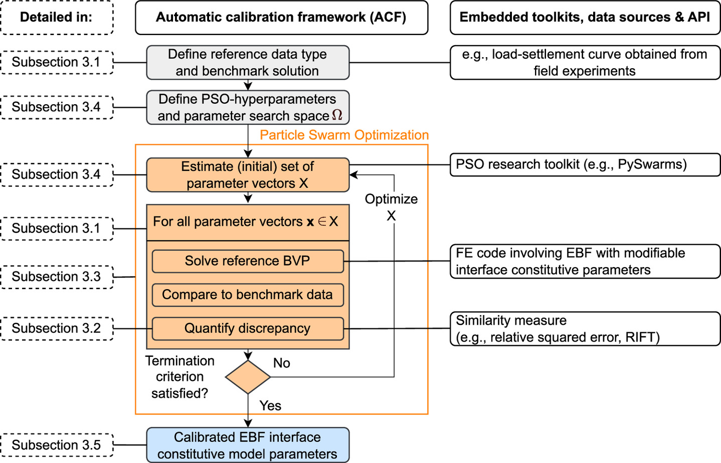
The basic idea of the proposed ACF is to calibrate the parameter vector , such that the results obtained with the EB-L* and EB-I* are as close as possible to the available benchmark data. This is conceptually realized by a global optimizer that operates in parallel on a set of parameter vectors denoted by . In the current version, the global optimizer allows for carrying out automatic calibration of on the basis of the single-objective optimization method (Papon et al. 2012), either using load–settlement curves or normal force distributions as reference data type. The ACF has been built on top of the commercial FE code Plaxis 3D (V2023.1, Bentley Systems) because it provides an application programming interface (API) to employ the EB-L* and EB-I* combined with an iterative optimization procedure to calibrate . Although this work is constrained to these two EBFs for brevity, it should be noted that the presented ACF can be easily extended to other EBFs and numerical codes, provided that they offer an API that allows one to control the ICMPs. The ACF is implemented using the object-oriented programming language Python (version 3.9.0), leveraged by scientific Python toolkits including PySwarms (version 1.3.0) (Miranda 2018), NumPy (version 1.24.4) (Harris et al. 2020), and SciPy (version 1.7.1) (Virtanen et al. 2020). According to the visual description in Fig. 5, algorithmic and implementational details of the ACF are subsequently explained in detail, followed by demonstration cases where the ACF is put into practice.
Working Scheme of the Optimal Parameter Vector Identification Strategy
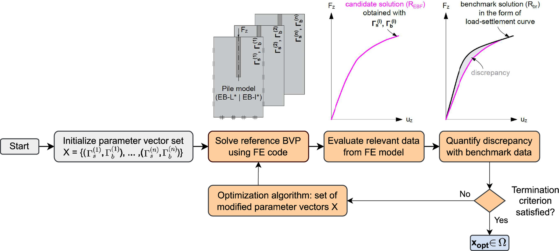
As a starting point, let us regard the numerically predicted pile response obtained with the EB-L* or EB-I*, denoted by , as a function of the unknown parameter vector (Fig. 4). From a mathematical point of view, finding the optimal parameter vector that minimizes the discrepancy between and the user-defined benchmark results can be expressed bywhere denotes the objective function that quantifies the discrepancy between and . The proposed ACF solves this bivariate minimization problem by adopting the so-called direct approach (Cividini et al. 1981), i.e., is identified by linking the results of parallel forward calculations to an optimization routine that iteratively updates the trial values in . Employing direct procedures to solve related back-analysis problems for the determination of suitable numerical parameters in geotechnical simulations has previously found wide application, for example, in large-scale mass movements (Meier et al. 2008, 2013), deep foundations (Pitteloud and Meier 2019), and deep excavations (Calvello and Finno 2004; Lin et al. 2015); for a comprehensive overview of relevant geotechnical application cases, interested readers can refer to Ebid (2021). In all cases, the authors agree on one issue: Provided that the forward solution of the employed simulation model captures the relevant properties of the benchmark problem with reasonable accuracy, the direct approach yields a valuable concept to increase the numerical fidelity of finite-element simulations. With reference to this work, this applies also for the determination of suitable values for and .
(6)
As visually explained in Fig. 6, the basic idea of the direct procedure adopted in this work concerns the identification of by solving a user-defined reference BVP involving an EBF in an iterative manner, followed by the successive evaluation of the objective function for on the basis of Eq. (6). In the current version, the suitability of the candidate solutions is assessed by comparing with , either in terms of a user-defined load–settlement curve or pile normal force distribution. Depending on the computed discrepancy between the benchmark data and the EBF simulation results, the trial values in are updated in parallel using a constrained optimization algorithm, i.e., is bound to a predefined search space representing the range of admissible values for and . This sequence of cycles continues until a termination criterion is fulfilled. With regard to the ACF configuration deployed in this work, the latter is defined by means of a user-defined maximum number of iteration cycles. Details concerning the mathematical expression of the objective function, optimization algorithm, and search space constraints are given in the next subsections.
Objective Function
The objective function driving the calibration of has to quantify the discrepancy between and based on Eq. (6) (Fig. 6). Moreover, it provides knowledge about the calibration state. The readers should notice, however, that convergence to the global optimum solution is not generally warranted. For example, this may be attributed to an inappropriate selection of the similarity measure (Machaček et al. 2022) or the incorporation of reference data types with limited physical meaning (Kadlíček et al. 2022).
To circumvent related issues in the calibration process, the evaluation of the objective function carried out in this work is restricted to the load–settlement ( ) curve (Fig. 6), a widely accepted representation of the physical pile behavior. In addition, the developed ACF offers the functionality to specify two conceptually different similarity measures to quantify the discrepancy between and , namely, the relative squared error ( ) (Jadon et al. 2022) and the robust and interpolation-free technique ( ) (Lin et al. 2015). Both similarity measures are graphically described in Fig. 7(a). The dimensionless constitutes a regression-type similarity measure that takes the general form:whereIn Eqs. (7) and (8), denotes the th reference data point, is the numerically predicted data point, and is the mean of reference data points. Since the reference and numerical data points are not generally expected to be aligned in one dimension (e.g., if the pile resistance values are sampled at different settlements) and may differ with respect to the number of available data points, the evaluation of requires the integration of an implicit regression procedure. The working principle of the underlying interpolation strategy adopted by the ACF is illustrated in Fig. 7(a). In this respect, it should be noted that the polynomial degree specified in the regression model should be specified with care because it may induce the common problem of underfitting or overfitting, leading to a poor approximation of the discrete data (Harrell et al. 1996) [Fig. 7(b)]. Alternatively, in cases where the discrete data describing the load–settlement curve is limited, it may be reasonable to deploy regularization techniques, such as Lasso regression (Ni et al. 2018a), to facilitate the evaluation of . However, it is pointed out that the use of related approaches may increase the complexity in the model selection due to the incorporation of additional hyperparameters, such as the shrinkage parameter associated with Lasso regression. In general, it is good practice to assess the suitability of the regression model employed in the ACF based on preliminary studies with varying . In the scope of this work, was found to be adequate to achieve a reasonable performance of the calibration procedure.
(7)
(8)
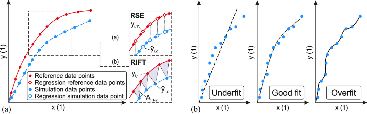
As an attractive alternative to prevent the use of a regression model, has been implemented as alternative similarity measure. Instead of computing purely distance-based measures between (artificially) aligned data points, accounts for the accumulated area of successive triangles formed by the two data sets under study [Fig. 7(a)]. Since can be classified as an interpolation-free similarity measure, its application is particularly advised in cases where interpolation may introduce significant errors in the approximation of the candidate curve, for example, in the case of data sets with various levels of data density. To date, however, the performance of has been investigated on the basis of a rather small number of demonstration cases documented in two publications (Lin et al. 2015; Hsieh et al. 2017), both of which provide limited discussion about potential limitations. For this purpose, part of the comparative studies presented in this work focus on how the selection of the similarity measure affects the performance of the ACF in the context of a single-pile problem.
Optimization Method
The computational efficiency of the ACF is mainly governed by the number of forward calculations required to approximate with sufficient accuracy. Accordingly, increasing the efficiency of the calibration procedure is equivalent to minimizing the number of iteration cycles (Fig. 6), notably at the cost of a higher parameter uncertainty. Consequently, it is imperative to select an optimization method that offers a reasonable balance between fast convergence and exploratory search, particularly because the objective functions may incorporate a number of locally optimal solutions. However, there is no general rule for selecting a proper optimization method since the performance depends on the problem characteristics that have to be assessed on a case-by-case basis (Meier and Schanz 2013).
In the present work, are iteratively updated employing the particle swarm optimization (PSO) algorithm, originally introduced by Kennedy and Eberhart (1995) and Shi and Eberhart (1998). The latter can be classified as the stochastic optimization algorithm (Wang et al. 2018), as opposed to deterministic algorithms that generally require gradient information with respect to the objective function; interested readers can refer to Hajihassani et al. (2018) for a comprehensive overview of PSO application cases in the field of geotechnical engineering, including hybrid configurations of PSO with conceptually different algorithms. Traditionally, PSO-based calibration frameworks greatly benefit from a high level of robustness, in the sense that broad variations in the hyperparameter selection do not prevent convergence (Clerc 2006), and quick exploration of large search spaces, possibly at the cost of a longer time consumption (Wang et al. 2018; Machaček et al. 2022). These features make the PSO algorithm particularly suitable for our low-dimensional characterization problem with two unknown calibration parameters and , which lacks profound numerical evidence about adequate value ranges for comparison.
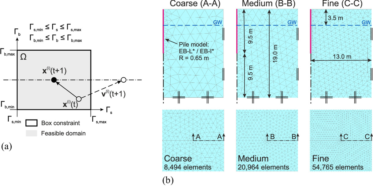
Adopting the terminology originally introduced by Kennedy and Eberhart (1995), the PSO operates on the so-called swarm involving particles, whereas the embedded interface stiffness multipliers belonging to the th particle may be interpreted as a candidate solution to the minimization problem stated in Eq. (6). In the present work, the swarm size is defined following empirical guidelines documented in Shi and Eberhart (1998). Starting from random initial positions, a velocity update method is used to simultaneously transfer the individual to updated positions at time step (Fig. 8):where denotes the positions of the th particle at time step , corresponding to the last iteration cycle, and is the velocity of the th particle at time step , expressed byTherein, and are positive acceleration coefficients used to scale the contribution of the cognitive and social components, respectively. and denote random scalars between 0 and 1 sampled from a uniform distribution which introduce a stochastic element to the algorithm. is the previous individual best position of the th particle and represents the previous global best positions of the swarm. is the inertia weight that controls the influence of the previous particle velocity in the course of exploratory search.
(9)
(10)
From Eq. (10), it can be inferred that the particle movement is governed by (1) its personal experience (cognitive component), (2) the experience of all particles in the swarm (social component) on the basis of the star topology [i.e., each particle disseminates information to all particles of the swarm; compare Ni and Deng (2013)], and (3) the inertia component in a role similar to friction in a physical setting [cf. Bratton and Kennedy (2007)]. In a biological context, this configuration emulates the social behavior of birds within a flock, particularly their ability to fly synchronously and continuously regroup in an optimal formation. A detailed discussion of the underlying social learning processes and the PSO hyperparameter characteristics, however, falls outside the scope of the present work. Details can be found in Engelbrecht (2007), Kennedy et al. (2009), and Helwig (2010).
In the current version of the ACF, the PSO hyperparameters documented in Table 1 are selected according to the specifications recommended in Eberhart and Shi (2000), originally derived on the basis of the constriction approach mathematically described in Clerc (1999) and Clerc and Kennedy (2002). The suitability of this hyperparameter set is additionally confirmed by empirical rules documented in Clerc (2006). Nevertheless, it should be noticed that the selection of PSO hyperparameters remains empirical to a large extent (Trelea 2003). This means that we may achieve a better optimization performance with a particular set of hyperparameter values. However, optimization experiments concerning the tuning of PSO hyperparameters, along with comparative studies employing alternative optimization algorithms, are beyond the scope of the present work and may be addressed in the future.
| (1) | (1) | (1) |
|---|---|---|
| 1.494 | 1.494 | 0.729 |
Search Space Constraints
The particle positions of the swarm are initialized uniformly at random in the search space (Fig. 6). To handle invalid particle positions in the course of the optimization, the so-called reflect position handling strategy (Helwig 2010) was adopted, as conceptually explained in Fig. 8(a). Essentially, both features require the definition of suitable box constraints to limit the search space region, being a delicate issue given the limited experience in the selection of . In general, box constraint specifications have a considerable influence on the performance of PSO search behavior: While an overly large may lead to a high variance between the different candidate solutions, the specification of considerably narrow tends to produce clusters at the boundaries (Machaček et al. 2022). Needless to say, the constrained PSO algorithm is unable to evaluate appropriate solutions to Eq. (6) if falls outside the feasible domain.
To evaluate suitable box constraints with adequate confidence, preliminary studies comprising 30 forward FE calculations with varying embedded interface stiffness multipliers were carried out employing the well-documented Alzey Bridge pile load test as a reference scenario (Sommer and Hambach 1974). Fig. 8(b) displays the adopted mesh configurations. Unless stated otherwise, the results are obtained with the medium mesh configuration comprising 20,964 tetrahedral solid FEs with quadratic element functions. The bored pile is modeled wished-in-place, that is, changes in the soil surrounding the pile induced by the installation process are not considered. The groundwater level is controlled by defined hydraulic pressure heads that are related to the groundwater table located 3.5 m below ground level. The numerical modeling parameters of the reference BVP, including the hardening soil small (HSS) (Benz 2007) constitutive model parameters of the soil domain conforming to slightly overconsolidated Frankfurt clay, combined with the material and geometrical parameters of the pile model are given in Table 2.
| Category | Parameter | Value |
|---|---|---|
| Pile parameters (constitutive model: linear elastic) | (kN/m ) | 25.0 |
| (MN/m ) | 10,000 | |
| (1) | 0.9 | |
| (m) | 9.5 | |
| (m) | 0.65 | |
| (1) | 0.2 | |
| Soil parameters (constitutive model: hardening soil small) | , (kN/m ) | 20.0 |
| (kN/m ) | 45,000 | |
| (kN/m ) | 27,150 | |
| (kN/m ) | 90,000 | |
| (1) | 1.0 | |
| (1) | 0.2 | |
| ( ) | 20.0 | |
| (kN/m ) | 20.0 | |
| POP (kN/m ) | 50.0 | |
| (kN/m ) | 100.0 | |
| (kN/m ) | 116,000 | |
| (1) | 0.00015 |
Source: Data from Granitzer and Tschuchnigg (2021).
All simulations were carried out utilizing the identical calculation phase sequence. The initial stress field was generated using the so-called K0 procedure. In this phase, only soil clusters are present and gravity loads are applied. These loads are derived from the soil unit weight and balanced by the effective vertical stresses in the soil. In analogy to Engin et al. (2007), where this pile problem has been adopted to validate an enhanced EB-L, the horizontal stresses are computed considering a preoverburden pressure kPa to realistically capture overconsolidation effects in the slightly overconsolidated Frankfurt clay. Interested readers can refer to Tschuchnigg (2012) for details concerning the influence of the adopted initial stress generation procedure on the yield surfaces of the HSS soil constitutive model. In the subsequent phases, the piles are activated and subjected to displacement-driven head-down loading.
A comparison of the experimental benchmark data obtained from field measurements (Sommer and Hambach 1974) and the load–settlement curves obtained using the EB-L* and EB-I* is plotted in Fig. 9. The readers should notice that the objective function , indicating the discrepancy between the results obtained from the measurements and the pile models, was evaluated by hand without using the ACF. From the results, three observations become striking: First, evaluated for the EB-I* is considerably smaller than 1 (i.e., the default value) and differs by around one order of magnitude compared to results obtained with the EB-L*. This clearly demonstrates that optimal embedded interface stiffness multipliers cannot be interchangeably used for both implementations and need to be assessed on a case-by-case basis. Second, the EB-L* produces mesh-dependent values with relatively high bandwidth, while the corresponding results obtained with the EB-I* remain almost constant in all cases considered. A third observation concerns the reproducibility of the benchmark solution: While the latter can be well captured by the EB-I*, irrespective of the mesh configuration, the EB-L* is unable to resemble the benchmark solution with the fine mesh discretization. An additional sensitivity study (not shown) has indicated similar but less pronounced tendencies with regard to .
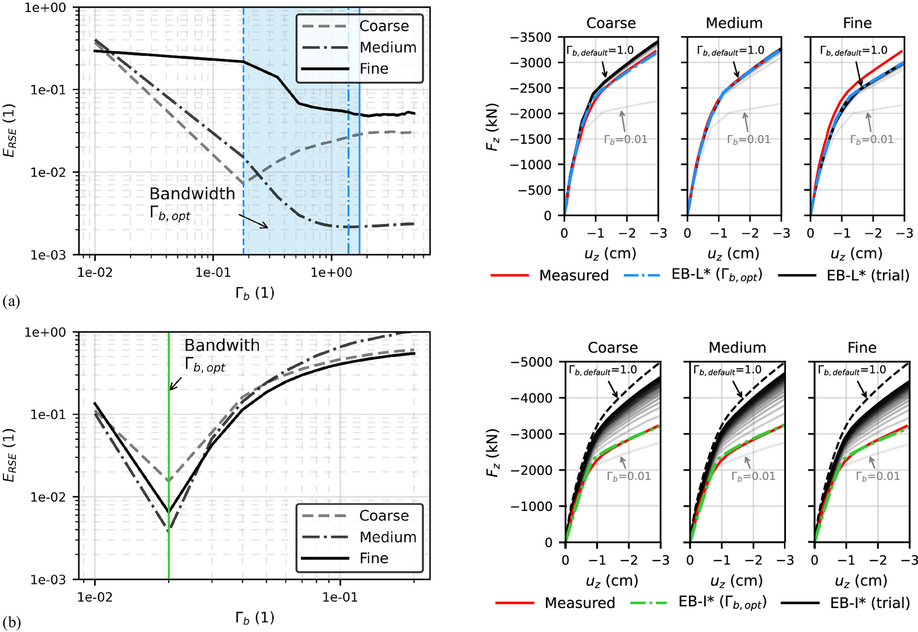
To some extent, the latter two observations can be attributed to the unwanted mesh size dependency inherent to the EB-L*, which is almost eliminated with the EB-I* due to the enhanced coupling scheme. It should be emphasized that this notable difference in the mesh sensitivity has an important implication with regard to the general applicability of calibration procedures for the determination of : While the results indicate a high level of reproducibility with regard to the EB-I*, the mesh size effect on the results obtained with the EB-L* leads to calibrated parameter sets that are only valid for one particular mesh topology deployed in the reference BVP; that is, calibrated ICMPs associated with the EB-L* tend to be mesh size dependent. From a practical point of view, this concern greatly disqualifies the application of calibration strategies, such as the ACF, to improve the numerical fidelity of large-scale BVPs involving a high number of EB-Ls* and strategic mesh refinement zones. For this purpose, the EB-L* is not considered in further analyses. In contrast, the results obtained with the EB-I* allow one to infer mesh size-independent box constraints. These are summarized in Table 3 and adopted for the ACF demonstration cases presented in the next sections.
| Parameter bounds | (1) | (1) |
|---|---|---|
| Min. | 0.001 | 0.001 |
| Max. | 0.1 | 0.1 |
Reference Solution
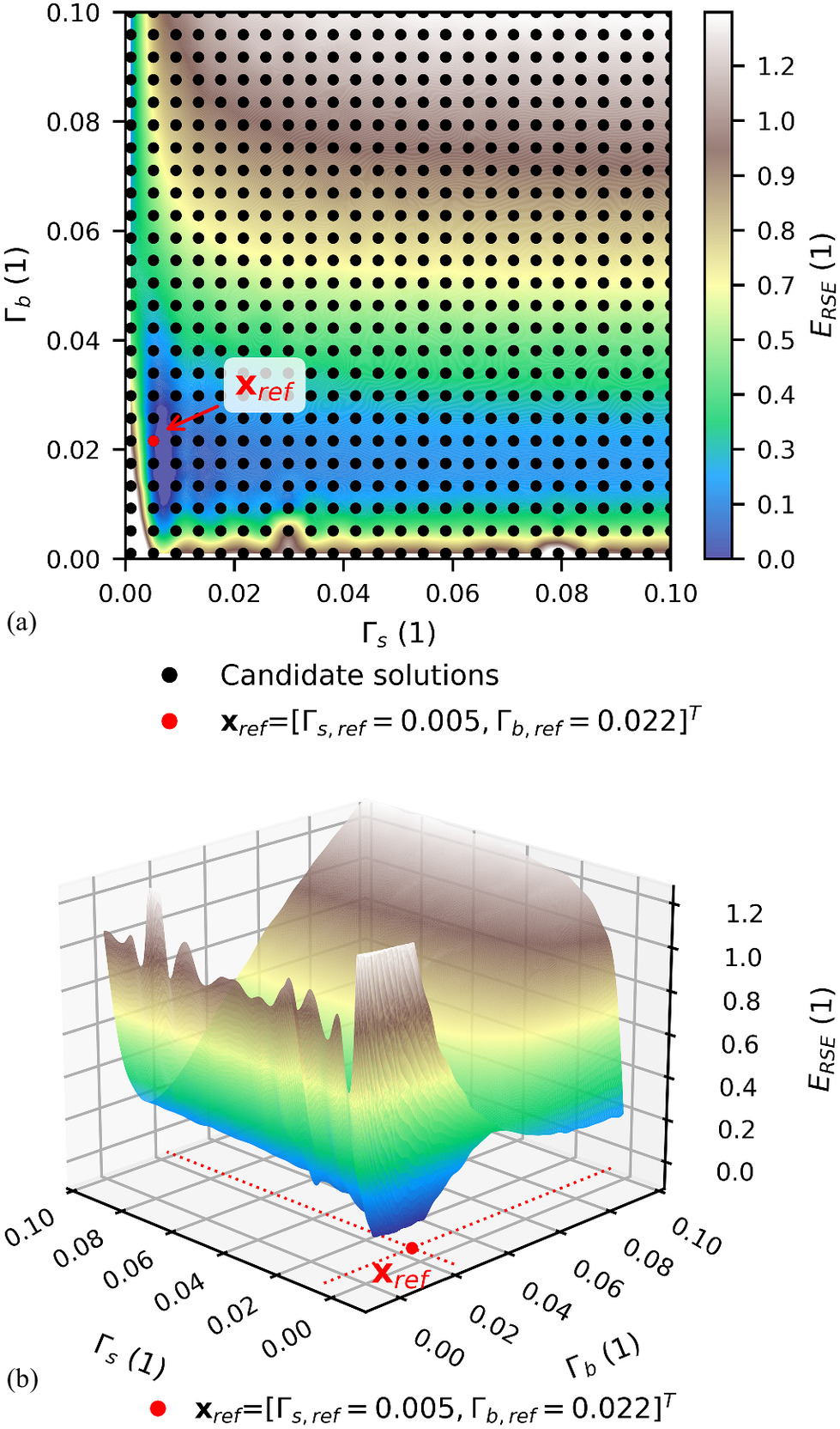
The validation of the proposed ACF necessitates a careful evaluation of the reference solution valid for the reference scenario. For this purpose, a grid search was adopted with evenly spaced intervals of the embedded interface stiffness multipliers. This involves taking a number of equally spaced trial solutions spread over the search space, thereby creating a total of 625 combinations to check. In Fig. 10(a), each candidate solution is represented by a black dot. As can be inferred from Fig. 10(b), the grid search-based reference solution with respect to is . In this regard, it is interesting to note that the reference parameter set significantly differs from the default values. This observation clearly underlines that the choice of suitable values for the ICMPs is imperative to achieve a high level of numerical fidelity in simulations involving EBFs. In the next section, the grid search-based reference solution serves as a validation basis to explore the capabilities of the ACF to identify optimal values for and .
Alzey Bridge Pile Load Test
This section examines the ability of the ACF to approximate associated with the Alzey Bridge pile load test reference scenario (Sommer and Hambach 1974). Focus is placed on the influence of the similarity measure and the role of the loading conditions. For each set of analyses, 20 iteration cycles were executed (Fig. 6).
Influence of Similarity Measure
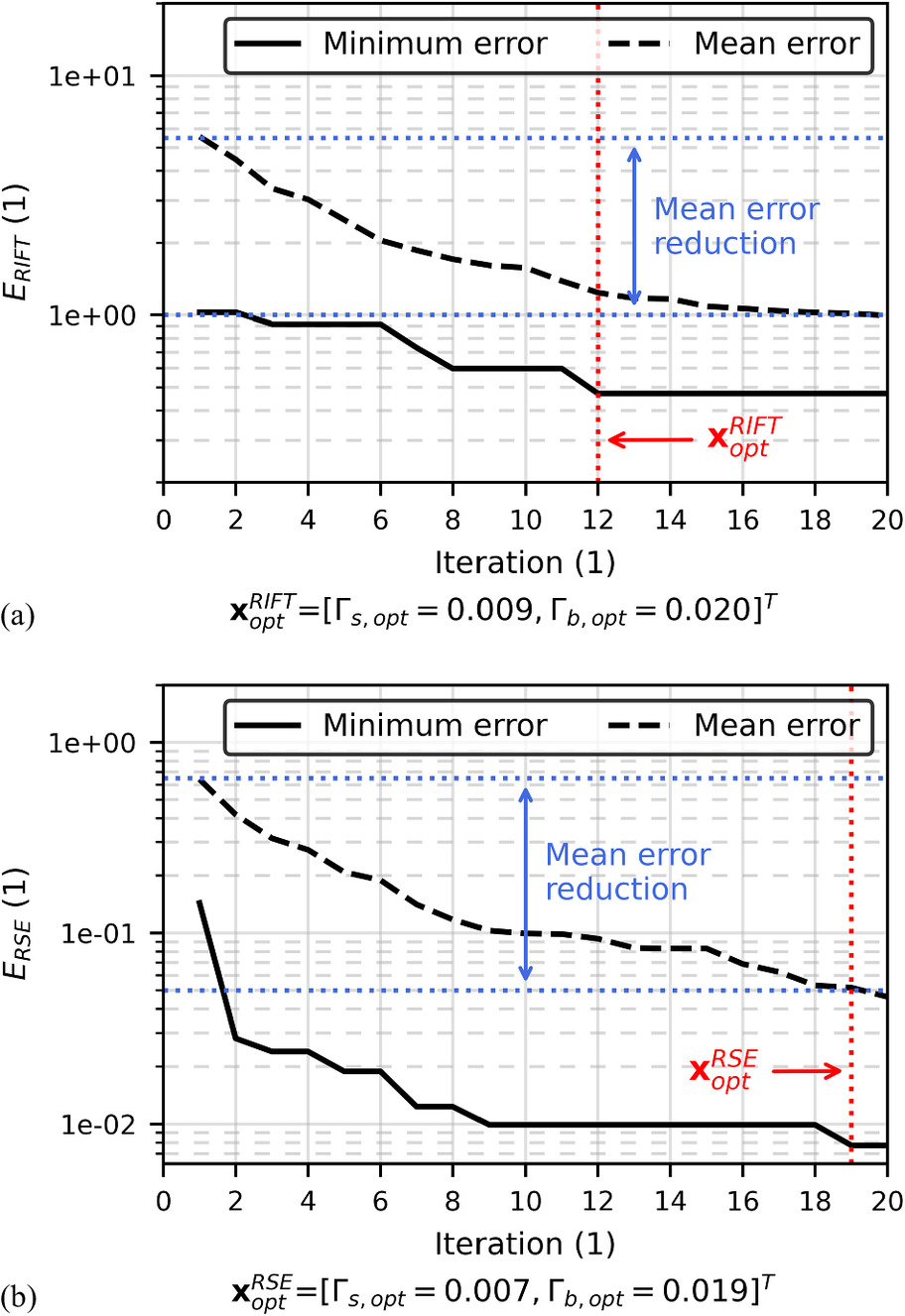
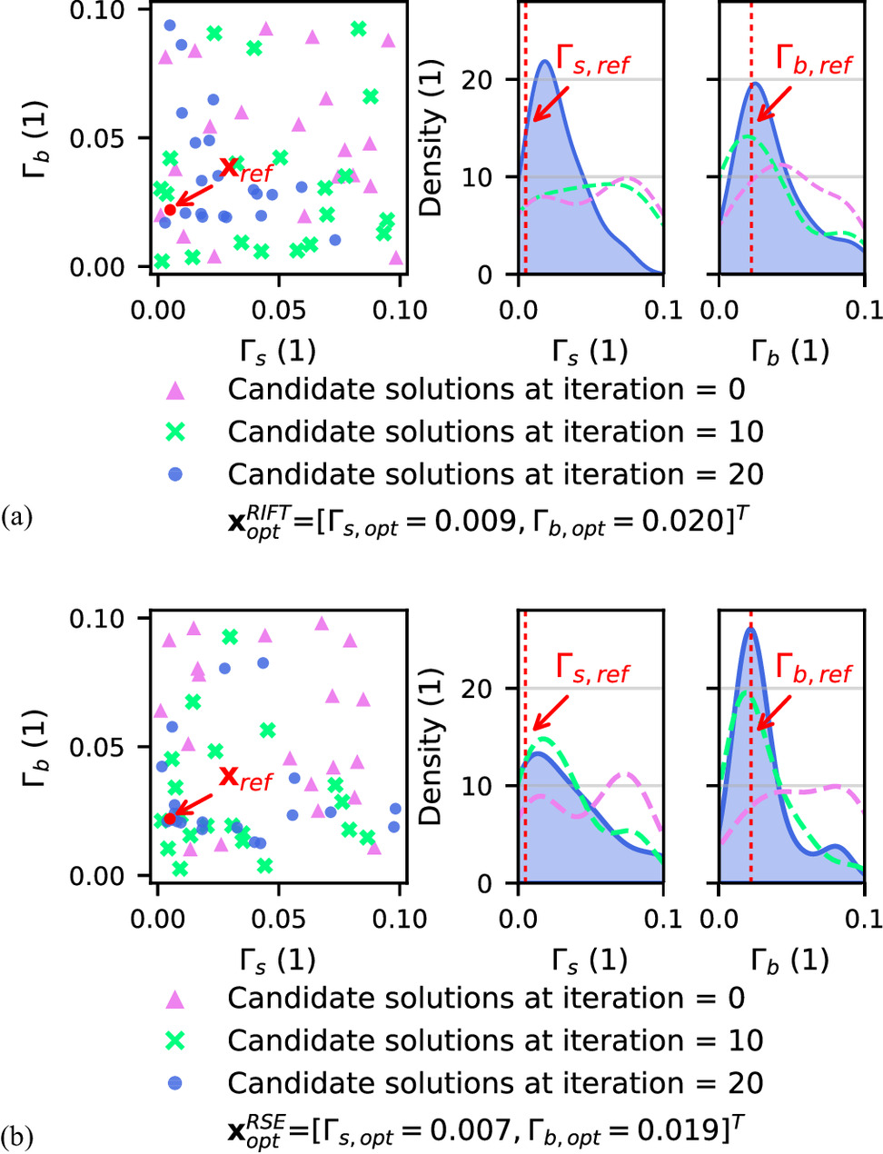
The first set of ACF-enabled analyses is executed employing the two different similarity measures (RSE and RIFT). Fig. 11 studies the convergence behavior with regard to the mean error (i.e., the mean objective function value of the swarm) and the minimum error (i.e., the best particle solution) found within each iteration cycle of the automatic calibration. Since the similarity measures have different mathematical definitions, a quantitative comparison in light of their influence on the performance of the ACF is not possible. Instead, the similarity measure has to produce curves with stagnant decrease and approximate with sufficient accuracy to be regarded as acceptable to solve the optimization task. In both cases, the convergence of the automatic calibration procedure is proven by a reduction of around 0.5–1.0 orders in the magnitude of the mean error. Moreover, it is demonstrated that the best solutions found by the ACF (i.e., and ) after 12 and 19 iteration cycles are in remarkable agreement with the grid search-based reference solution reported in Fig. 10(c).
The rate of convergence observed in Fig. 11 is largely controlled by the sensitivity of the objective function to the calibration parameters (i.e., and ), whereas a higher level of sensitivity leads to a faster convergence. As an intuitive measure to quantify the parameter sensitivity and describe the relevance of each calibration parameter to achieve a good fit of the simulations with the measured load–settlement curve, it is common practice (Mendez et al. 2021) to compare the coefficient of variation (COV) with respect to the tested calibration parameters. This metric is defined as the ratio of the standard deviation normalized by the mean. As can be seen from the results documented in Table 4, the COV shows similar values in the range of 66.5%–74.6% for each embedded interface stiffness multiplier, irrespective of the similarity measure. This implies that the adequate estimation of and , respectively, is of similar importance to achieve a good fit of the numerically derived EB-I* load–settlement curve with the measured reference data.
| Similarity measure | (1) | (1) | COV (%) | (1) | (1) | COV (%) |
|---|---|---|---|---|---|---|
| RIFT | 0.043 | 0.028 | 66.5 | 0.040 | 0.028 | 69.9 |
| RSE | 0.039 | 0.029 | 74.6 | 0.036 | 0.026 | 72.3 |
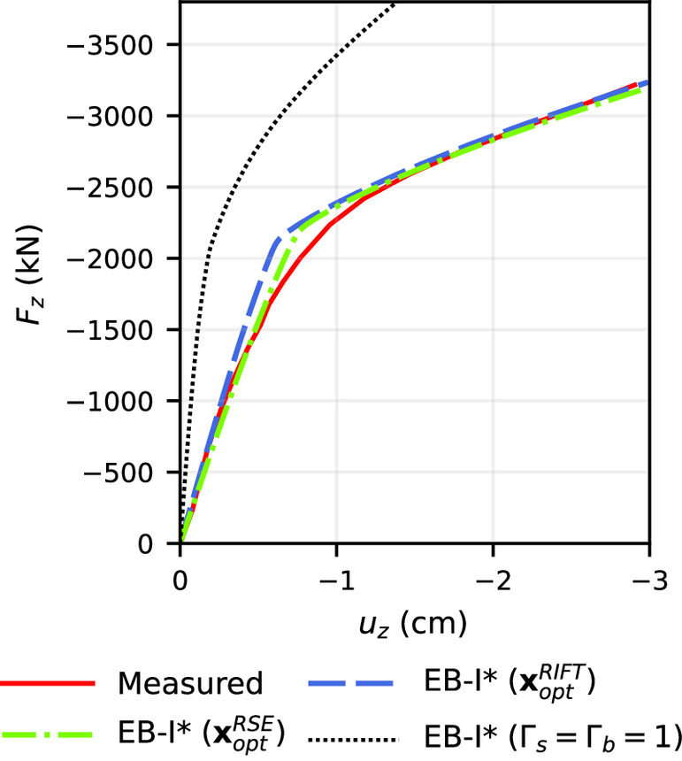
From a user perspective, the most relevant aspect in the performance assessment of the ACF is probably the comparison of the measured load–settlement curve with the simulation results. In this context, Fig. 12 displays the effect of using calibrated values for and . A visual inspection of the results obtained with and confirms the significantly improved agreement with the measured load–settlement curve compared to the EB-I* simulations with noncalibrated (default) values for and . From this observation, it becomes obvious that the numerical predictions obtained with the EB-I* greatly benefit from the ACF.
Despite the good agreement of EB-I* predictions obtained with calibrated ICMPs observed in Fig. 12, the computed COV values may be considered relatively high. This can be attributed to the wide limits selected for the (unknown) search space constraints (Table 3) and the lack of physical interpretation of and , both of which represent fitting parameters that control the kinematic behavior of (see Fig. 4). This implies a certain degree of parameter uncertainty that is, to some extent, reflected in the nonnegligible variance of and in the scatter plots illustrated in Fig. 13, showing the mutual particle distributions after 1, 10, and 20 iteration cycles. A lower scatter in the candidate solutions and hence an improved performance of the ACF in terms of reproducibility could be achieved by tuning the PSO hyperparameters in Table 1 or by selecting narrower bounds with respect to the search space constraints. The latter option, however, would require the examination of search space constraints on a case-by-case basis, representing a time-consuming task that impedes general employment of the ACF in practice. Considering the corresponding Gaussian kernel density estimates of the calibration parameters presented in Fig. 13, however, this appears nonessential because the results clearly indicate the desired gradual movement of particles toward . This concern is substantiated by the concentration of high-density regions close to and and holds for both similarity measures. Although the results infer the desired gradual increase of density peaks around and with increasing iterations cycle number and hence an adequate convergence of the calibration procedure toward the optimal solution, it appears somewhat premature to claim general applicability of the termination criterion adopted in this study. This aspect is therefore revisited in the next section considering an isolated pile in multilayer soil as a reference scenario.
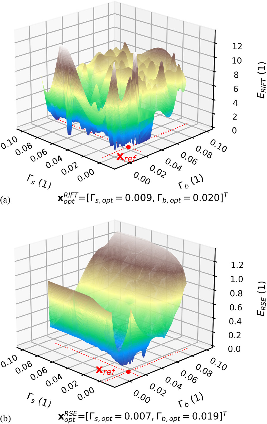
The objective function topologies shown in Fig. 14 shed light on an additional interesting detail concerning the capabilities of the different similarity measures: While shows a relatively smooth pattern with a global minimum close to , produces a clearly nondifferentiable function with multiple local minima. It could therefore be expected that the use of leads to a relatively reduced stability of the ACF. This can be explained by the different mathematical descriptions of the discrepancy between the measured load–settlement curve and the simulation results, particularly because is more sensitive to large deviations between corresponding pairs of reference and numerically predicted data points. From the previous discussion, it can be concluded that the ACF is more prone to the occurrence of unwanted effects during the calibration procedure, such as premature convergence and local optimization (Qian et al. 2021), if is selected as a similarity measure. Consequently, automatic calibration by means of is recommended and selected for further analyses.
Influence of Loading Magnitude
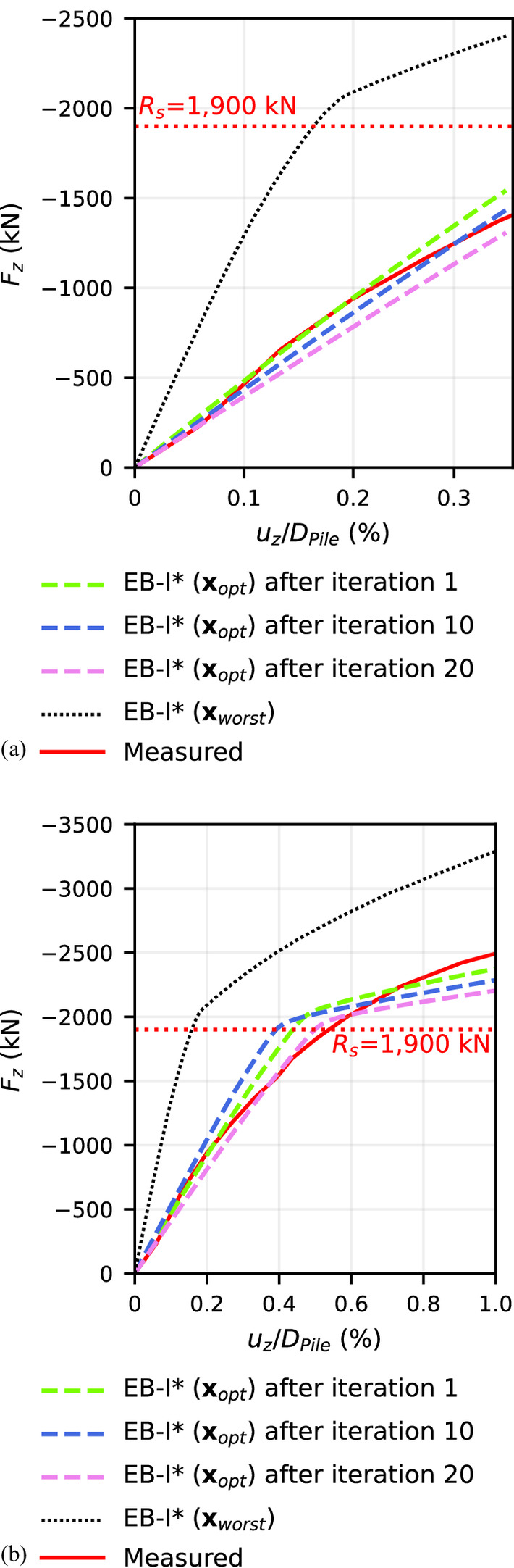
The results presented in the previous subsection are obtained considering the full load–settlement measuring interval cm of the field test. Nevertheless, it needs to pointed out that this specification is user-defined and may vary depending on the available reference data. This step is comparable to the selection of experimental value ranges in oedometric and triaxial tests required for the calibration of constitutive model parameters (Knabe et al. 2013; Kadlíček et al. 2022). Considering the simplified numerical description of the soil–structure contact inherent to EBFs visually desribed in Fig. 3, in combination with the bivariate nature of the calibration problem underlying the ACF, it is nearly impossible that the EB-I* matches the measured load–settlement curve in a perfect manner. Even if the perfect interface constitutive model for the EB-I* existed, scattering of experimental results, measurement errors and remaining mesh size effects (albeit significantly reduced compared to the EB-L*) would prevent a perfect fit. From a calibration point of view, this is likely to result in nonunique solutions for that are specific to the user provided load–settlement range. It is noteworthy that the accurate anticipation of relevant loading ranges for large-scale simulations, however, is subject to human influences, especially when dealing with practical problems at early project phases. This appears to be a step backward because it is the human factor that is pursued to become dispensable by the development of the ACF. Nevertheless, to this date, this path is inevitable [compare Machaček et al. (2022)].
To assess the impact of the selected loading conditions on the variability of , the automatic calibration procedure was executed using two loading magnitudes: , to capture the end of the initial linear region in the load–settlement curve (Chen and Fang 2009), and . As could be expected from the aforementioned discussion, the loading conditions influence the calibration results, with the optimal parameter vectors computed after 20 iteration cycles being and (Fig. 15). Correspondingly, the loading magnitude has a notable effect on the objective function topology. Moreover, it can be seen that yields similar values, as opposed to values that are sensitive to the loading magnitude. This is attributed to the different contributions of and , respectively, to the mobilization of EB-I* pile resistance (Fig. 4). As long as the ultimate shaft resistance reported at around kN (Sommer and Hambach 1974) is not reached, the pile resistance mobilization rate of an EB-I* is dominated by . Consequently, values specified for are of subordinate importance to achieve a good fit with the measurements because this loading magnitude falls inside the initial loading range. In contrast, a notable base resistance is mobilized with . This has the consequence that the parameter uncertainty of simultaneously decreases with increasing loading magnitude.
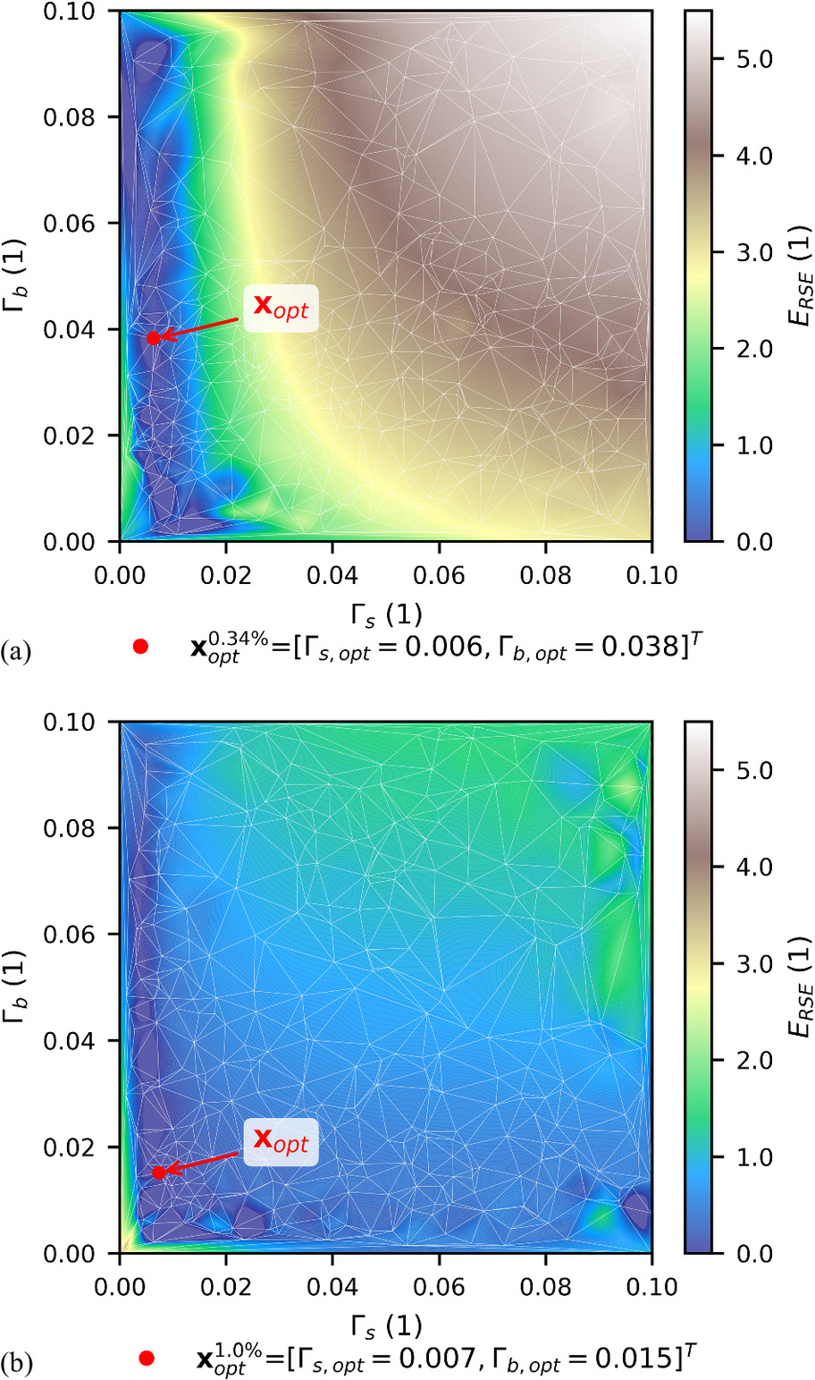
Despite the variance in the calibrated parameters triggered by a varying loading magnitude, Fig. 16 underlines that the ACF is a powerful tool to increase the credibility of simulations where the EB-I* is used for the modeling of pile-type structures. It should be noted, however, that the loading magnitude provided as input to the ACF may influence the calibration results, particularly with respect to the base resistance mobilization, i.e., overly small values may yield inaccurate estimates of . It is therefore advised to provide reference data with sufficiently high loading magnitude, such that the maximum loading levels experienced by the calibrated EB-I* in the envisaged large-scale BVP are captured.
Sony Center Pile Load Test
In this section, the ACF is deployed to a pile in multilayered soil problem. For this purpose, the Sony Center Static pile load test (Anthogalidis 1996) executed in Berlin sand was considered as a reference scenario. The focus of this study was to assess the convergence behavior in light of the maximum iteration cycle number used as a termination criterion.
Finite-Element Model
All geometrical and constitutive model parameters utilized in this study were adopted from Wehnert and Vermeer (2004). Fig. 17 illustrates the discretized domain of the reference boundary value problem comprising 21,631 tetrahedral solid FEs with quadratic element functions. The soil stratification is assumed horizontally layered and consists of medium dense sand (Sand 1) underpinned by a dense sand (Sand 2) formation with a narrow interlayer of Marl; the corresponding hardening soil model (Schanz et al. 1999) and Mohr–Coulomb constitutive model parameters are listed in Table 5, along with the pile properties applied for the EB-I*. The calculation phase sequence is identical to the one utilized in the Alzey Bridge pile load test analysis scenario.
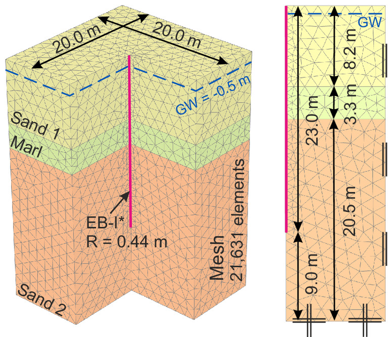
| Category | Parameter | Value |
|---|---|---|
| Pile parameters (constitutive model: linear elastic) | (kN/m ) | 25.0 |
| (MN/m ) | 10,000 | |
| (1) | 0.3/1.0 | |
| (m) | 23.0 | |
| (m) | 0.44 | |
| (1) | 0.2 | |
| Soil parameters Sand 1/Sand 2 (constitutive model: hardening soil) | , (kN/m ) | 20.0/21.0 |
| (kN/m ) | 45,000/60,000 | |
| (kN/m ) | 45,000/60,000 | |
| (kN/m ) | 180,000/270,000 | |
| ( ) | 32.5/37.5 | |
| ( ) | 2.5/7.5 | |
| (kN/m ) | 0.1 | |
| (1) | 0.6 | |
| (1) | 0.2 | |
| (kN/m ) | 100.0 | |
| Soil parameters Marl (constitutive model: Mohr–Coulomb) | , (kN/m ) | 21.0 |
| (kN/m ) | 200,000 | |
| ( ) | 27.5 | |
| (kN/m ) | 30.0 | |
| (1) | 0.33 |
Source: Data from Wehnert and Vermeer (2004).
Influence of Iteration Cycle Number
As of now, there is little experience regarding the choice of the maximum iteration cycle number required to ensure satisfactory convergence of the optimal parameter vector to the sought solution. It should be noticed that this setting has a crucial impact on both, the time consumption of the calibration procedure and the quality of the identified calibration parameters. To provide insight into the relevance of the ACF termination criterion, the maximum iteration cycle number is increased to 50, as opposed to the previous examples where 20 iteration cycles are considered. Fig. 18(a) collects the main results of the automatic calibration as function of the iteration cycle number. In accordance with the numerical evidence obtained from the Alzey Bridge pile load test reference scenario, the results indicate reasonable convergence rates of the calibration procedure, underlined by a reduction of more than one magnitude of order in the mean error. Fig. 18(b) allows for a more detailed analysis with respect to the quality of the calibration parameters identified by the best particle position in the swarm (i.e., ). It can be inferred that the first 25 iteration cycles yield a notable scatter in the objective function, followed by a relatively constant distribution until the termination criterion is triggered. In the present case, this means that the contribution of iteration cycle numbers higher than 25 to the increase in quality of the identified calibration parameters can be regarded insignificant.
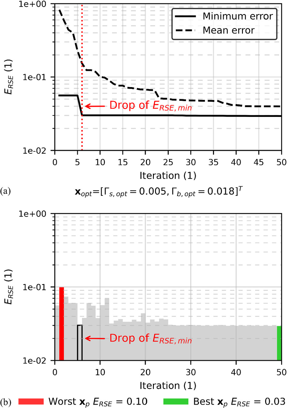
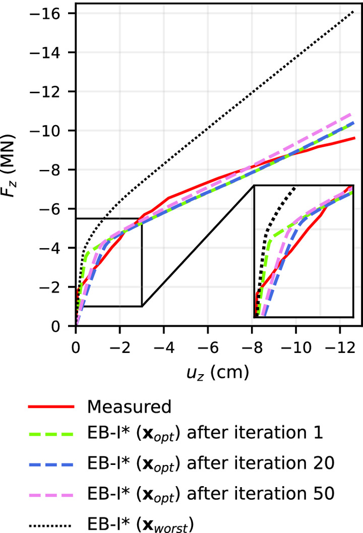
From the results in Fig. 18(b), it can be also deduced that the best fit of the EB-I* simulations with the measured load–settlement curve, corresponding to the particle position with the smallest value found during the iterative search (i.e., ), is qualitatively comparable to the results obtained with in Iteration cycle 6. This is particularly reflected by the sharp drop of the minimum error in Fig. 18(a). The readers should notice, however, that this observation is largely triggered by the initialization of the particle positions and velocities and hence should not be generalized to reduce the runtime of the automatic calibration because the final solution quality may be affected in an adverse manner [cf. Helwig (2010)]. It is therefore essential to notice that the formulation of general guidelines regarding the maximum number of iteration cycles is out of reach for this work because it depends on numerous of factors, including but not restricted to the initial configuration of the swarm, box constraints, similarity measures, and reference data. In addition, it may be advised to introduce a supplemental termination criterion that defines a minimum lowering of required after a number of iteration cycles to proceed with the iterative search (Meier et al. 2008). To date, we can only suggest to produce a study similar to the one depicted in Fig. 18, in combination with a detailed visual inspection of critical areas in the load–settlement curves to ensure calibration parameters with sufficient accuracy at reasonable computational expense. In the present case, the numerical predictions depicted in Fig. 19 show that the simulated EB-I* load–settlement curve is considerably improved between Iteration cycles 1 and 20, particularly in the initial loading range. Inversely, higher iteration cycles tend to yield an insignificant change in the predicted EB-I* response but affect the computational expense associated with the automatic calibration in an unfavorable manner.
Pile Group Analysis
So far, it is not clear whether the improved credibility of numerical predictions obtained with calibrated parameter sets scales to large-scale BVPs involving multiple EB-Is*. To this end, the performance of the ACF is analyzed in the light of a pile group problem. This section describes the reference scenario, followed by the calibration of and using the ACF. Comparative studies display the effect of using calibrated interface constitutive model parameters in the pile group analysis and highlight the role of the reference BVP adopted by the ACF.
Investigated Scenario
Fig. 20 illustrates the problem geometry and loading conditions adopted from Franza and Sheil (2021). In their work, a stick-slip EBF (Granitzer et al. 2024) has been used for the pile modeling, notably without providing details about the interaction domain geometry and relevant ICMPs that control the pile displacement behavior prior to the onset of plastic slip. Table 6 lists the linear–elastic pile and HSS soil parameters adopted for Vienna sand, originally published by Tschuchnigg and Schweiger (2010). In analogy to Franza and Sheil (2021), the ACF performance was examined based on comparisons with a numerical benchmark solution where the piles are modeled by means of the SFEA, in which zero-thickness interface elements (Day and Potts 1994) are introduced at the pile–soil interfaces with the same properties of the soil. From the displayed mesh topologies, it can be observed that the FE number and hence the number of unknowns that has to be solved are substantially reduced with the EB-I* model. The elevated rigid cap is modeled weightless and attached to the piles by means of fixed connections. It is pointed out that the cap is not in contact with the underlying soil. This geometrical configuration renders the BVP particularly suitable for examining the ACF performance because the structural response is fully controlled by interactions between the piles and the soil that are, in turn, bound to the values selected for and . The calculation phase sequence is identical to the ones utilized in the previous analysis scenarios. A salient difference is the selected point displacement magnitude imposed on the cap center that is defined in accordance with design guidelines commonly used in pile group analyses (Witt 2018).
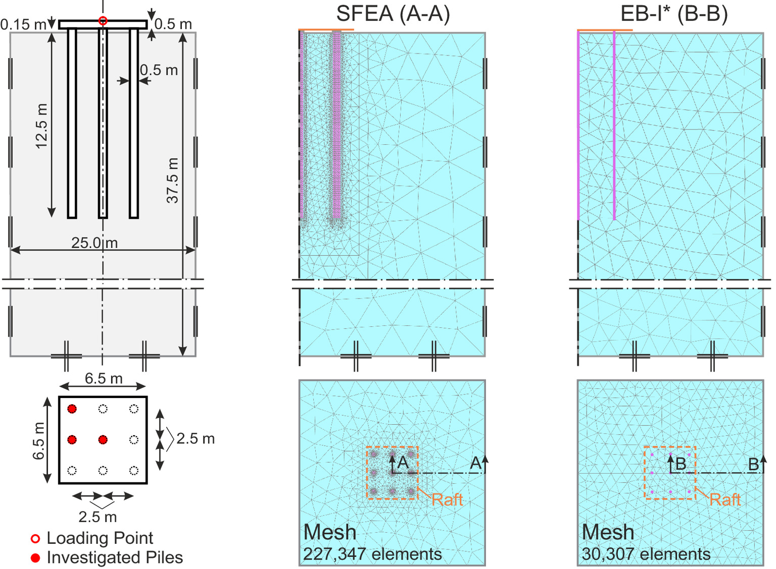
| Category | Parameter | Value |
|---|---|---|
| Pile parameters (constitutive model: linear elastic) | (kN/m ) | 25.0 |
| (MN/m ) | 10,000 | |
| (1) | 0.9 | |
| (m) | 12.5 | |
| (m) | 0.25 | |
| (1) | 0.2 | |
| Soil parameters (constitutive model: hardening soil small) | , (kN/m ) | 20.0 |
| (kN/m ) | 25,000 | |
| (kN/m ) | 25,000 | |
| (kN/m ) | 62,500 | |
| (1) | 0.65 | |
| (1) | 0.2 | |
| ( ) | 32.5 | |
| ( ) | 2.5 | |
| (kN/m ) | 2.0 | |
| POP (kN/m ) | 600.0 | |
| (kN/m ) | 100.0 | |
| (kN/m ) | 78,125 | |
| (1) | 0.0002 |
Source: Data from Tschuchnigg (2012).
Parameter Calibration
In accordance with the studies presented in the two preceding sections, and are calibrated based on a single-pile reference BVP (Fig. 21). The constitutive model parameters, pile geometry and loading conditions, are identical to the piled cap reference scenario documented in Fig. 20 and Table 6. In the absence of field measurements, however, the benchmark load–settlement curve was recovered from the numerical SFEA benchmark model. The PSO hyperparameters and search space constraints considered in the ACF were adopted from Tables 1 and 3, respectively. To ensure a reasonable convergence of the automatic calibration, was used as a similarity measure.
As a key output of the calibration procedure, Fig. 21 shows the EB-I* results evaluated with the best parameter vector observed during 20 iteration cycles and the load–settlement curve of the numerical benchmark model. A comparison with the EB-I* results corresponding to the worst parameter vector highlights, on the one hand, the remarkable ability of the EB-I* to emulate the SFEA benchmark response, provided that adequate IMCPs are selected. On the other hand, it confirms the high potential of the adopted ACF to increase the credibility of EB-I* predictions by solving this calibration task. In the next subsection, we investigate whether these observations also extend to the piled cap problem involving numerous piles.
Foundation Displacements
To date, the majority of simulations involving EB-Is* reported in the literature has been constrained to single-pile analyses. In this study, the EB-I* is for the first time used to analyze a capped pile group (Fig. 20). To assess the significance of using calibrated ICMPs to achieve EB-I* predictions with reasonable accuracy, the simulations were carried out with default and calibrated parameter sets, that is, and .
Fig. 22 illustrates the pile load–settlement curves obtained with the EB-I* models and the numerical SFEA benchmark. It can be inferred from the results that the load-bearing behavior of the piles differs with the respective pile position, whereas the corner pile displays the highest pile resistance mobilization rates and the central pile shows the least. This observed tendency is typical for low-settlement bored pile groups and becomes more determinant with increasing pile spacing, pile number, pile slenderness ratio ( ), and soil stiffness; interested readers can refer to Poulos and Davis (1980) for details. Although not observed in this study, it should be noted for completeness that settlement magnitudes could lead to a reversal of this tendency due to interlocking effects. The results presented in Fig. 22 additionally highlight the high relevance of an adequate selection of ICMPs. While the default parameter set results in an overly stiff response of the piles, the remarkable agreement of the calibrated EB-I* results with the numerical SFEA benchmark observed along the full range of loading is striking.
With reference to the selection of the reference BVP in Fig. 6, the ACF could also be theoretically deployed using a full representation of the piled cap, leading to a considerable increase in computational expense for the calibration procedure. However, the results presented in this study underline the generalizability of the ACF in identifying optimal parameter sets based on single-pile reference BVPs, in the sense that they are equally applicable to large-scale BVPs involving multiple EB-Is*. Readers should note that this is an important observation of this study because it allows one to restrain the computational effort during the calibration procedure to stay beyond practical limits.
Conclusions
This work demonstrates that the credibility of numerical simulations involving EBFs is significantly controlled by the choice of their ICMPs. To date, the selection of adequate values remains unclear to a large extent. This distinct lack of research decreases the confidence in the results obtained with EBFs and has motivated the development of an ACF based on box-constrained PSO. The following conclusions can be drawn from this analysis:
•
The numerical description of the soil–structure interaction behavior associated with state-of-the art EBFs builds on simplifying assumptions that are often disregarded in practice. Essentially, the accurate representation of local field variables within the local zone of shearing lies beyond the capabilities of EBFs. This concern implies that their ICMPs should be calibrated based on global response analyses employing full-scale boundary value problems, instead of using stress point observations that are commonly adopted for the calibration of soil constitutive model parameters.
•
It is demonstrated that the applicability of calibration procedures is closely related to the mesh size sensitivity of the EBF. With reference to the EBFs used in this work, it is shown that the calibrated ICMPs obtained for the embedded beam with interaction line (EB-L*) proposed by Tschuchnigg and Schweiger (2015) are nonunique because they are valid for one particular mesh only. This limitation impedes the deployment of calibration procedures to determine IMCPs for the EB-L*. In contrast, the embedded beam with interaction surface (EB-I*) detailed in Granitzer et al. (2024) produces consistent calibrated parameter sets that remain valid for various mesh discretizations.
•
The design of the ACF is flexible in the sense that it allows for the definition of various benchmark data types, stochastic optimization methods based on PSO, similarity measures, and box constraints. The suitability of different configurations of these variables is critically examined and complemented with practical recommendations. The configuration adopted in this manuscript is successfully validated based on three different pile problems.
•
Two similarity measures are implemented to quantify the discrepancy between the benchmark data and EBF prediction and hence the quality of the selected ICMPs. Contrary to the relative squared error, the RIFT proposed by Lin et al. (2015) produces a clearly nondifferentiable function with multiple local minima. To the authors’ best knowledge, this artifact is reported for the first time, significantly undermining the suitability of RIFT for related calibration tasks.
•
To assess the applicability of the proposed ACF, three demonstration cases with piles modeled by means of the EB-I* are presented. In all cases, the results confirm the high relevance of an adequate ICMP selection. Moreover, it is highlighted that the ACF is very effective in solving the underlying calibration task.
•
It is demonstrated that, for the considered capped pile group boundary value problem, ICMPs calibrated based on single-pile analyses can be effectively applied to large-scale problems involving multiple piles. This observation increases the potential for take-up in engineering practice because it restrains the calibration effort to stay beyond practical limits.
Although the demonstration cases presented in this work are constrained to ICMPs of the EB-I*, the ACF can be seamlessly transferred to related calibration tasks associated with different EBFs and finite-element codes. However, depending on the selected calibration parameters, it may be required to modify the PSO hyperparameters and search space constraints to achieve both reasonable convergence rates and adequate calibration results.
Data Availability Statement
All data, models, or code that support the findings of this study are available from the corresponding author upon reasonable request.
Acknowledgments
Supported by TU Graz Open Access Publishing Fund.
Notation
The following symbols are used in this paper:
- base area (m ) and circumference (m) of virtual beam geometry;
- beam nodes and virtual solid nodes;
- acceleration coefficients and inertia weight (PSO hyperparameters);
- pile diameter (m);
- medium value of the particle size distribution (m);
- error obtained with robust and interpolation-free technique;
- relative squared error;
- EB-L
- embedded beam FE with interaction line (1D-to-3D coupling scheme);
- EB-L
- EB-L after Tschuchnigg and Schweiger (2015);
- EB-I
- embedded beam FE with interaction surface (2D-to-3D coupling scheme);
- EB-I
- EB-I after Granitzer et al. (2024);
- vertical pile resistance (kN);
- average shear stiffness of TSFE (kN/m );
- element function associated with the th node of TSFE;
- number of solid nodes belonging to TSFE;
- number of TSFE at the EB-I interaction surface;
- virtual beam radius (m);
- benchmark response and numerically predicted response;
- ultimate shaft resistance (kN);
- random scalar values between 0 and 1;
- traction component in the axial direction (kN/m, kN/m );
- shear zone thickness (m);
- , ,
- displacement vectors of beam and solid domain/ th node of TSFE (m);
- interface, local shear, and pile displacements (m), respectively;
- relative and soil displacements (m), respectively;
- vertical pile head settlement (m);
- velocities of the th particle at time steps and , respectively;
- global weight of the peripheral interaction surface segment;
- parameter vector with values of embedded interface stiffness multipliers;
- positions of the th particle at time steps and , respectively;
- global and individual best particle positions, respectively;
- position vector of the th coupling point (m);
- position vector of the th node belonging to TSFE (m);
- optimal parameter vectors with calibrated values of and identified by ACF;
- optimal parameter vector for and , respectively;
- optimal parameter vectors considering RIFT and RSE, respectively;
- grid search-based parameter vector with reference values of and ;
- embedded interface stiffness multipliers considered at the base and shaft, respectively;
- interaction zones at the base (b) and shaft (s), respectively;
- peripheral interaction surface segment;
- embedded interface stiffness multipliers associated with EB-L* and EB-I*, respectively;
- mean value;
- position vectors in the local reference system of TSFE;
- standard deviation;
- search space; and
- 3D solid (s) and 1D beam (b) domains, respectively.
References
Abbas, Q., G. Kim, I. Kim, D. Kyung, and J. Lee. 2021. “Lateral load behavior of inclined micropiles installed in soil and rock layers.” Int. J. Geomech. 21 (6): 1–13. https://doi.org/10.1061/(ASCE)GM.1943-5622.0002021.
Abo-Youssef, A., M. S. Morsy, A. El Ashaal, and Y. M. El Mossallamy. 2021. “Numerical modelling of passive loaded pile group in multilayered soil.” Innovative Infrastruct. Solutions 6 (2): 1–13. https://doi.org/10.1007/s41062-021-00464-6.
Al-abboodi, I., and T. T. Sabbagh. 2019. “Numerical modelling of passively loaded pile groups.” Geotech. Geol. Eng. 37 (4): 2747–2761. https://doi.org/10.1007/s10706-018-00791-z.
Anthogalidis, A. 1996. “Pfahlprobebelastungen im Berliner Sand.” Vertieferarbeit, Institute of Geotechnical Engineering, Technical Univ. of Darmstadt.
Banerjee, R., S. Bandyopadhyay, A. Sengupta, and G. R. Reddy. 2020. “Settlement behaviour of a pile raft subjected to vertical loadings in multilayered soil.” Geomech. Geoeng. 17 (1): 1–15.
Benz, T. 2007. “Small-strain stiffness of soils and its numerical consequences.” Ph.D. thesis, Institute for Geotechnics, Univ. of Stuttgart.
Bratton, D., and J. Kennedy. 2007. “Defining a standard for particle swarm optimization.” In Proc., 2007 IEEE Swarm Intelligence Symposium, 120–127. Piscataway, NJ: IEEE Computer Society.
Cai, X. 2003. “Overlapping domain decomposition methods.” In Advanced topics in computational partial differential equations, edited by T. J. Barth, M. Griebel, D. E. Keyes, R. M. Nieminen, D. Roose, T. Schlick, H. P. Langtangen, and A. Tveito, 57–95. Vol. 33 of Lecture Notes in Computational Science and Engineering. Berlin: Springer.
Calvello, M., and R. J. Finno. 2004. “Selecting parameters to optimize in model calibration by inverse analysis.” Comput. Geotech. 31 (5): 410–424. https://doi.org/10.1016/j.compgeo.2004.03.004.
Chang, T. Y., H. Taniguchi, and W. F. Chen. 1987. “Nonlinear finite element analysis of reinforced concrete panels.” J. Struct. Eng. 113 (1): 122–140. https://doi.org/10.1061/(ASCE)0733-9445(1987)113:1(122).
Chen, Y.-J., and Y.-C. Fang. 2009. “Critical evaluation of compression interpretation criteria for drilled shafts.” J. Geotech. Geoenviron. Eng. 135 (8): 1056–1069. https://doi.org/10.1061/(ASCE)GT.1943-5606.0000027.
Chen, Z., P. Ni, X. Zhu, and G. Mei. 2022. “Using boundary transform method to solve geotechnical problems with mixed-type boundary conditions.” J. Geotech. Geoenviron. Eng. 148 (12): 06022013.
Cividini, A., L. Jurina, and G. Gioda. 1981. “Some aspects of ‘characterization’ problems in geomechanics.” Int. J. Rock Mech. Min. Sci. Geomech. 18 (6): 487–503. https://doi.org/10.1016/0148-9062(81)90513-1.
Clerc, M. 1999. “The swarm and the queen: Towards a deterministic and adaptive particle swarm optimization.” In Proc., 1999 Congress on Evolutionary Computation, 1951–1957. Piscataway, NJ: IEEE Service Center.
Clerc, M. 2006. Particle swarm optimization. London and Newport Beach, CA: ISTE.
Clerc, M., and J. Kennedy. 2002. “The particle swarm—Explosion, stability, and convergence in a multidimensional complex space.” IEEE Trans. Evol. Comput. 6 (1): 58–73. https://doi.org/10.1109/4235.985692.
Day, R. A., and D. M. Potts. 1994. “Zero thickness interface elements—Numerical stability and application.” Int. J. Numer. Anal. Methods Geomech. 18 (10): 689–708. https://doi.org/10.1002/nag.v18:10.
de Gennaro, V., R. Frank, and I. Said. 2008. “Finite element analysis of model piles axially loaded in sands.” Riv. Ital. Geotec. 2: 44–62.
DeJong, J. T., and Z. J. Westgate. 2009. “Role of initial state, material properties, and confinement condition on local and global soil-structure interface behavior.” J. Geotech. Geoenviron. Eng. 135 (11): 1646–1660. https://doi.org/10.1061/(ASCE)1090-0241(2009)135:11(1646).
DeJong, J. T., D. J. White, and M. F. Randolph. 2006. “Microscale observation and modeling of soil-structure interface behavior using particle image velocimetry.” Soils Found. 46 (1): 15–28. https://doi.org/10.3208/sandf.46.15.
Di Prisco, C., L. Flessati, and D. Porta. 2020. “Deep tunnel fronts in cohesive soils under undrained conditions: A displacement-based approach for the design of fibreglass reinforcements.” Acta Geotech. 15 (4): 1013–1030. https://doi.org/10.1007/s11440-019-00840-8.
Eberhart, R. C., and Y. Shi. 2000. “Comparing inertia weights and constriction factors in particle swarm optimization.” In Proc., 2000 Congress on Evolutionary Computation, 84–88. Piscataway, NJ: IEEE Service Center.
Ebid, A. M. 2021. “35 years of (AI) in geotechnical engineering: State of the art.” Geotech. Geol. Eng. 39 (2): 637–690. https://doi.org/10.1007/s10706-020-01536-7.
Engelbrecht, A. P. 2007. Computational intelligence: An introduction. 2nd ed. Chichester, UK: Wiley.
Engin, H. K., and R. B. J. Brinkgreve. 2009. “Investigation of pile behaviour using embedded piles.” In Proc., 17th Int. Conf. on Soil Mechanics and Geotechnical Engineering, edited by M. Hamza, M. Shahien, and Y. El-Mossallamy, 1189–1192. Amsterdam, Netherlands: IOS Press.
Engin, H. K., R. B. J. Brinkgreve, and E. G. Septanika. 2007. “Improved embedded beam elements for the modelling of piles.” In Numerical models in geomechanics, edited by G. N. Pande. London: Taylor & Francis.
Engin, H. K., R. B. J. Brinkgreve, and A. F. van Tol. 2015. “Approximation of pile installation effects: A practical tool.” Proc. Inst. Civ. Eng. Geotech. Eng. 168 (4): 319–334. https://doi.org/10.1680/geng.14.00064.
Engin, H. K., E. G. Septanika, and R. B. J. Brinkgreve. 2008. “Estimation of pile group behavior using embedded piles.” In Proc., 12th Int. Conf. on Computer Methods and Advances in Geomechanics, edited by M. N. Jadhav, 3231–3238. New York: Curran.
Esmaeili, M., M. G. Nik, and F. Khayyer. 2013. “Experimental and numerical study of micropiles to reinforce high railway embankments.” Int. J. Geomech. 13 (6): 729–744. https://doi.org/10.1061/(ASCE)GM.1943-5622.0000280.
Franza, A., and B. Sheil. 2021. “Pile groups under vertical and inclined eccentric loads: Elastoplastic modelling for performance based design.” Comput. Geotech. 135: 104092. https://doi.org/10.1016/j.compgeo.2021.104092.
German Geotechnical Society, 2014. Recommendations on piling (EA-Pfähle). 2nd ed. Ernst & Sohn Series on Geotechnical Engineering. Berlin: Wilhelm Ernst & Sohn.
Goudarzi, M., and A. Simone. 2019. “Discrete inclusion models for reinforced composites: Comparative performance analysis and modeling challenges.” Comput. Methods Appl. Mech. Eng. 355: 535–557. https://doi.org/10.1016/j.cma.2019.06.026.
Granitzer, A., F. Tschuchnigg, W. Summerer, R. Galler, and T. Stoxreiter. 2021. “Construction of a railway tunnel above the main drainage tunnel of Stuttgart using the cut-and-cover method.” Bauingenieur 96 (5): 156–164. https://doi.org/10.37544/0005-6650-2021-05.
Granitzer, A.-N., and H. Felic. 2022. “Das embbedded beam element mit explizierter Interaktionsoberfläche—Optimierte Modellierung linearer Strukturelemente.” In 37. Baugrundtagung, edited by German Geotechnical Society, 45–54. Essen, Germany: Deutsche Gesellschaft fr Geotechnik.
Granitzer, A.-N., M. J. Rebhan, and F. Tschuchnigg. 2022. “Influence of reaction system on uplift behaviour of micropiles subjected to static pullout.” In Field measurements in geomechanics, edited by A. M. Ridley. London: International Society for Soil Mechanics and Geotechnical Engineering.
Granitzer, A.-N., and F. Tschuchnigg. 2021. “Practice-oriented validation of embedded beam formulations in geotechnical engineering.” Processes 9 (10): 1739. https://doi.org/10.3390/pr9101739.
Granitzer, A.-N., and F. Tschuchnigg. 2023a. “Behaviour of embedded beam formulations under dynamic loading.” In Proc., 5th Int. Conf. on New Developments in Soil Mechanics and Geotechnical Engineering, edited by C. Atalar and F. Çinicioğlu, 353–361. Vol. 305 of Lecture Notes in Civil Engineering. Cham: Springer.
Granitzer, A.-N., and F. Tschuchnigg. 2023b. “Finite element formulations for implicit beam-to-solid coupling: Numerical obstacles and solution strategies.” In Proc., 10th European Conference on Numerical Methods in Geotechnical Engineering (NUMGE2023), edited by L. Zdravkovic, S. Kontoe, D. M. G. Taborda, and A. Tsiampousi, 1–6. London: International Society for Soil Mechanics and Geotechnical Engineering.
Granitzer, A.-N., and F. Tschuchnigg. 2023c. “On the use of embedded beam formulations for the numerical analysis of deep foundations.” In Challenges and innovations in geomechanics, edited by M. Barla, A. Di Donna, D. Sterpi, and A. Insana, 307–314. Vol. 288 of Lecture Notes in Civil Engineering. Cham: Springer.
Granitzer, A.-N., F. Tschuchnigg, S. Hosseini, and S. Brasile. 2024. “Insight into numerical characteristics of embedded finite elements for pile–type structures employing an enhanced formulation.” Int. J. Numer. Anal. Methods Geomech. 48 (1): 223–249. https://doi.org/10.1002/nag.v48.1.
Hajihassani, M., D. Jahed Armaghani, and R. Kalatehjari. 2018. “Applications of particle swarm optimization in geotechnical engineering: A comprehensive review.” Geotech. Geol. Eng. 36 (2): 705–722. https://doi.org/10.1007/s10706-017-0356-z.
Harrell, F. E., K. L. Lee, and D. B. Mark. 1996. “Multivariable prognostic models: Issues in developing models, evaluating assumptions and adequacy, and measuring and reducing errors.” Stat. Med. 15 (4): 361–387. https://doi.org/10.1002/(SICI)1097-0258(19960229)15:4%3C361::AID-SIM168%3E3.0.CO;2-4.
Harris, C. R., et al. 2020. “Array programming with NumPy.” Nature 585 (7825): 357–362. https://doi.org/10.1038/s41586-020-2649-2.
Helwig, S. 2010. “Particle swarms for constrained optimization.” Ph.D. thesis, Technische Fakultät, Friedrich-Alexander-Universität Erlangen-Nürnberg.
Henke, S., and J. Grabe. 2008. “Numerical investigation of soil plugging inside open-ended piles with respect to the installation method.” Acta Geotech. 3 (3): 215–223. https://doi.org/10.1007/s11440-008-0079-7.
Hsieh, Y.-M., P. H. Dang, and H.-D. Lin. 2017. “How small strain stiffness and yield surface affect undrained excavation predictions.” Int. J. Geomech. 17 (3): 1–13. https://doi.org/10.1061/(ASCE)GM.1943-5622.0000753.
Hu, L., and J. Pu. 2004. “Testing and modeling of soil-structure interface.” J. Geotech. Geoenviron. Eng. 130 (8): 851–860. https://doi.org/10.1061/(ASCE)1090-0241(2004)130:8(851).
Jadon, A., A. Patil, and S. Jadon. 2022. “A comprehensive survey of regression based loss functions for time series forecasting.” Preprint, submitted November 5, 2022. http://arxiv.org/abs/2211.02989.
Jürgens, H., P. Vogel, S. Henke, and J. Grabe. 2022. “Zur numerischen berechnung der globalen standsicherheit von bauwerken im boden.” Geotechnik 45 (3): 155–169. https://doi.org/10.1002/gete.v45.3.
Kadlíček, T., T. Janda, M. Šejnoha, D. Mašín, J. Najser, and Š. Beneš. 2022. “Automated calibration of advanced soil constitutive models. Part II: Hypoplastic clay and modified cam-clay.” Acta Geotech. 17 (8): 3439–3462. https://doi.org/10.1007/s11440-021-01435-y.
Kavitha, P. E., K. S. Beena, and K. P. Narayanan. 2016. “A review on soil–structure interaction analysis of laterally loaded piles.” Innovative Infrastruct. Solutions 1 (1): 1–14. https://doi.org/10.1007/s41062-016-0015-x.
Kennedy, J., and R. Eberhart. 1995. “Particle swarm optimization.” In Proc., Int. Conf. on Neural Networks, 1942–1948. Piscataway, NJ: IEEE.
Kennedy, J., R. C. Eberhart, and Y. Shi. 2009. Swarm intelligence. 8th ed. San Francisco: Morgan Kaufmann.
Knabe, T., M. Datcheva, T. Lahmer, F. Cotecchia, and T. Schanz. 2013. “Identification of constitutive parameters of soil using an optimization strategy and statistical analysis.” Comput. Geotech. 49: 143–157. https://doi.org/10.1016/j.compgeo.2012.10.002.
Lee, K. M., and Z. R. Xiao. 2001. “A simplified nonlinear approach for pile group settlement analysis in multilayered soils.” Can. Geotech. J. 38 (5): 1063–1080. https://doi.org/10.1139/t01-034.
Lin, H.-D., P. H. Dang, and Y.-M. Hsieh. 2015. “Rift: Robust and interpolation-free technique for objective functions in geotechnical inverse analysis.” Comput. Geotech. 64: 96–104. https://doi.org/10.1016/j.compgeo.2014.11.008.
Lo, S. 2014. “A study in an attempt to use embedded pile structure elements to simulate soil nail structures in PLAXIS 2D 2012 and 3D 2012.” In Numerical methods in geotechnical engineering, edited by M. Hicks, R. Brinkgreve, and A. Rohe, 765–769. London: CRC Press.
Machaček, J., P. Staubach, C. E. G. Tavera, T. Wichtmann, and H. Zachert. 2022. “On the automatic parameter calibration of a hypoplastic soil model.” Acta Geotech. 17 (11): 5253–5273. https://doi.org/10.1007/s11440-022-01669-4.
Martinez, A., J. D. Frost, and G. L. Hebeler. 2015. “Experimental study of shear zones formed at sand/steel interfaces in axial and torsional axisymmetric tests.” Geotech. Test. J. 38 (4): 1–18. https://doi.org/10.1520/GTJ20140266.
Meier, J., M. Moser, M. Datcheva, and T. Schanz. 2013. “Numerical modeling and inverse parameter estimation of the large-scale mass movement Gradenbach in Carinthia (Austria).” Acta Geotech. 8 (4): 355–371. https://doi.org/10.1007/s11440-013-0211-1.
Meier, J., W. Schaedler, L. Borgatti, A. Corsini, and T. Schanz. 2008. “Inverse parameter identification technique using PSO algorithm applied to geotechnical modeling.” J. Artif. Evol. Appl. 2008: 1–14.
Meier, J., and T. Schanz. 2013. “Benchmarking of optimization algorithms.” In Computational methods in tunneling and subsurface engineering, edited by G. Meschke, 1–8. Freiburg, Germany: Aedificatio Publishers.
Mendez, F. J., A. Pasculli, M. A. Mendez, and N. Sciarra. 2021. “Calibration of a hypoplastic model using genetic algorithms.” Acta Geotech. 16 (7): 2031–2047. https://doi.org/10.1007/s11440-020-01135-z.
Miranda, L. J. V. 2018. “Pyswarms: A research toolkit for particle swarm optimization in Python.” J. Open Source Software 3 (21): 433. https://doi.org/10.21105/joss.
Muir Wood, D. 2002. “Some observations of volumetric instabilities in soils.” Int. J. Solids Struct. 39 (13): 3429–3449. https://doi.org/10.1016/S0020-7683(02)00166-X.
Ni, P., S. Mangalathu, and Y. Yi. 2018a. “Fragility analysis of continuous pipelines subjected to transverse permanent ground deformation.” Soils Found. 58 (6): 1400–1413. https://doi.org/10.1016/j.sandf.2018.08.002.
Ni, P., I. D. Moore, and W. A. Take. 2018b. “Numerical modeling of normal fault-pipeline interaction and comparison with centrifuge tests.” Soil Dyn. Earthquake Eng. 105: 127–138. https://doi.org/10.1016/j.soildyn.2017.10.011.
Ni, Q., and J. Deng. 2013. “A new logistic dynamic particle swarm optimization algorithm based on random topology.” Sci. World J. 2013: 1–8. https://doi.org/10.1155/tswj.v2013.1.
Ninić, J., J. Stascheit, and G. Meschke. 2014. “Beam-solid contact formulation for finite element analysis of pile-soil interaction with arbitrary discretization.” Int. J. Numer. Anal. Methods Geomech. 38 (14): 1453–1476. https://doi.org/10.1002/nag.v38.14.
Oliveria, D., and P. K. Wong. 2011. “Use of embedded pile elements in 3D modelling of piled-raft foundations.” Aust. Geomech. J. 46 (3): 9–19.
Papon, A., Y. Riou, C. Dano, and P.-Y. Hicher. 2012. “Single-and multi-objective genetic algorithm optimization for identifying soil parameters.” Int. J. Numer. Anal. Methods Geomech. 36 (5): 597–618. https://doi.org/10.1002/nag.v36.5.
Peng, S. Y., C. W. W. Ng, and G. Zheng. 2014. “The dilatant behaviour of sand-pile interface subjected to loading and stress relief.” Acta Geotech. 9 (3): 425–437. https://doi.org/10.1007/s11440-013-0216-9.
Phillips, D. V., and O. C. Zienkiewicz. 1976. “Finite element non-linear analysis of concrete structures.” Proc. Inst. Civ. Eng. 61 (1): 59–88.
Pitteloud, L., and J. Meier. 2019. “High-frequency monitoring results of a piled raft foundation under wind loading.” Int. J. Geotech. Geol. Eng. 13 (3): 90–102.
Potts, D. M., and L. Zdravkovic. 2001. Finite element analysis in geotechnical engineering: Application. 1st ed. London: Thomas Telford.
Potyondy, J. G. 1961. “Skin friction between various soils and construction materials.” Géotechnique 11 (4): 339–353.
Poulos, H. G., and E. H. Davis. 1980. Pile foundation and design. Hoboken, NJ: Wiley.
Qian, J., W. Xu, L. Mu, and A. Wu. 2021. “Calibration of soil parameters based on intelligent algorithm using efficient sampling method.” Underground Space 6 (3): 329–341. https://doi.org/10.1016/j.undsp.2020.04.002.
Randolph, M. F., and C. P. Wroth. 1978. “Analysis of deformation of vertically loaded piles.” J. Geotech. Eng. Div. 104 (12): 1465–1488. https://doi.org/10.1061/AJGEB6.0000729.
Sadek, M., and I. Shahrour. 2004. “A three-dimensional embedded beam element for reinforced geomaterials.” Int. J. Numer. Anal. Methods Geomech. 28 (9): 931–946. https://doi.org/10.1002/nag.v28:9.
Scarfone, R., M. Morigi, and R. Conti. 2020. “Assessment of dynamic soil-structure interaction effects for tall buildings: A 3D numerical approach.” Soil Dyn. Earthquake Eng. 128: 1–14. https://doi.org/10.1016/j.soildyn.2019.105864.
Schanz, T., P. A. Vermeer, and P. G. Bonnier. 1999. “The hardening soil model: Formulation and verification.” In Beyond 2000 in computational geotechnics, edited by R. B. J. Brinkgreve, 281–296. Oxfordshire, UK: Routledge.
Scott, D. W. 1992. Multivariate density estimation: Theory, practice, and visualization. New York: Wiley.
Sheil, B., and B. A. McCabe. 2012. “Predictions of friction pile group response using embedded piles in PLAXIS.” In Proc., 3rd Int. Conf. on New Developments in Soil Mechanics and Geotechnical Engineering, edited by Turkish National Committee of SMGE, 679–686. Nicosia, Turkey: Near East Univ.
Shi, Y., and R. Eberhart. 1998. “A modified particle swarm optimizer.” In Proc., 1998 IEEE Int. Conf. on Evolutionary Computation Proceedings. IEEE World Congress on Computational Intelligence (Cat. No. 98TH8360), 69–73. Piscataway, NJ: IEEE.
Smulders, C. M., S. Hosseini, and R. Brinkgreve. 2019. “Improved embedded beam with interaction surface.” In Proc., 17th European Conf. on Soil Mechanics and Geotechnical Engineering, edited by H. Sigursteinsson, S. Erlingsson, and B. Bessason, 1048–1055. Reykjavík, Iceland: Committee of Conference (COC).
Sommer, H., and P. Hambach. 1974. “Großpfahlversuche im Ton für die Talbrücke Alzey.” Bauingenieur 49: 310–317.
Staubach, P., J. Machaček, M. C. Moscoso, and T. Wichtmann. 2020. “Impact of the installation on the long-term cyclic behaviour of piles in sand: A numerical study.” Soil Dyn. Earthquake Eng. 138: 1–14. https://doi.org/10.1016/j.soildyn.2020.106223.
Staubach, P., J. Machaček, and T. Wichtmann. 2022. “Novel approach to apply existing constitutive soil models to the modelling of interfaces.” Int. J. Numer. Anal. Methods Geomech. 46 (7): 1241–1271. https://doi.org/10.1002/nag.v46.7.
Steinbrecher, I., N. Hagemeyer, C. Meier, and A. Popp. 2022a. “A consistent mixed-dimensional coupling approach for 1D Cosserat beams and 2D solid surfaces.” Preprint, submitted October 28, 2022. https://doi.org/10.48550/arXiv.2210.16010.
Steinbrecher, I., M. Mayr, M. J. Grill, J. Kremheller, C. Meier, and A. Popp. 2020. “A mortar-type finite element approach for embedding 1D beams into 3D solid volumes.” Comput. Mech. 66 (6): 1377–1398. https://doi.org/10.1007/s00466-020-01907-0.
Steinbrecher, I., A. Popp, and C. Meier. 2022b. “Consistent coupling of positions and rotations for embedding 1D Cosserat beams into 3D solid volumes.” Comput. Mech. 69 (3): 701–732. https://doi.org/10.1007/s00466-021-02111-4.
Tafili, M., A. Ganal, T. Wichtmann, and O. Reul. 2023. “On the AVISA model for clay—Recommendations for calibration and verification based on the back analysis of a piled raft.” Comput. Geotech. 154: 105126. https://doi.org/10.1016/j.compgeo.2022.105126.
Tradigo, F., F. Pisanò, and C. Di Prisco. 2016. “On the use of embedded pile elements for the numerical analysis of disconnected piled rafts.” Comput. Geotech. 72: 89–99. https://doi.org/10.1016/j.compgeo.2015.11.005.
Trelea, I. C. 2003. “The particle swarm optimization algorithm: Convergence analysis and parameter selection.” Inf. Process. Lett. 85 (6): 317–325. https://doi.org/10.1016/S0020-0190(02)00447-7.
Truty, A. 2023. “Nonlocal FEM modeling of piles as beam elements embedded within 3D continuum.” Eng. Struct. 277: 1–14. https://doi.org/10.1016/j.engstruct.2022.115460.
Tschuchnigg, F. 2012. “3D finite element modelling of deep foundations employing an embedded pile formulation.” Ph.D. thesis, Institute of Soil Mechanics, Foundation Engineering and Computational Geotechnics, Graz Univ. of Technology.
Tschuchnigg, F., and H. F. Schweiger. 2010. “Study of a complex deep foundation system using 3D finite element analysis.” In Numerical methods in geotechnical engineering, edited by S. Nordal and T. Benz, 40–46. Leiden, Netherlands: CRC Press.
Tschuchnigg, F., and H. F. Schweiger. 2015. “The embedded pile concept—Verification of an efficient tool for modelling complex deep foundations.” Comput. Geotech. 63: 244–254. https://doi.org/10.1016/j.compgeo.2014.09.008.
Turello, D. F., F. Pinto, and P. J. Sánchez. 2016. “Embedded beam element with interaction surface for lateral loading of piles.” Int. J. Numer. Anal. Methods Geomech. 40 (4): 568–582. https://doi.org/10.1002/nag.v40.4.
Turello, D. F., F. Pinto, and P. J. Sánchez. 2017. “Three dimensional elasto-plastic interface for embedded beam elements with interaction surface for the analysis of lateral loading of piles.” Int. J. Numer. Anal. Methods Geomech. 41 (6): 859–879. https://doi.org/10.1002/nag.v41.6.
Turello, D. F., P. J. Sánchez, P. J. Blanco, and F. Pinto. 2018. “A variational approach to embed 1D beam models into 3D solid continua.” Comput. Struct. 206: 145–168. https://doi.org/10.1016/j.compstruc.2018.05.008.
Uesugi, M., and H. Kishida. 1986. “Influential factors of friction between steel and dry sands.” Soils Found. 26 (2): 33–46. https://doi.org/10.3208/sandf1972.26.2_33.
Virtanen, P., et al. 2020. “SciPy 1.0: Fundamental algorithms for scientific computing in Python.” Nat. Methods 17 (3): 261–272. https://doi.org/10.1038/s41592-019-0686-2.
Wang, D., D. Tan, and L. Liu. 2018. “Particle swarm optimization algorithm: An overview.” Soft Comput. 22 (2): 387–408. https://doi.org/10.1007/s00500-016-2474-6.
Wehnert, M., and P. A. Vermeer. 2004. “Numerische Simulation von Probebelastungen an Großbohrpfählen.” In Bauen in Boden und Fels, edited by H. Schad. Ostfildern, Germany: Technischen Akademie Esslingen.
Witt, K. J., ed. 2018. Grundbau-Taschenbuch: Teil 3. Gründungen und geotechnische Bauwerke. 8th ed. Berlin and München: Ernst.
Information & Authors
Information
Published In

International Journal of Geomechanics
Volume 24 • Issue 11 • November 2024
Copyright
This work is made available under the terms of the Creative Commons Attribution 4.0 International license, https://creativecommons.org/licenses/by/4.0/.
History
Received: Jul 17, 2023
Accepted: May 30, 2024
Published online: Sep 4, 2024
Published in print: Nov 1, 2024
Discussion open until: Feb 4, 2025
ASCE Technical Topics:
- Beams
- Calibration
- Constitutive relations
- Engineering fundamentals
- Engineering materials (by type)
- Foundations
- Geotechnical engineering
- Materials engineering
- Mathematics
- Measurement (by type)
- Models (by type)
- Numerical models
- Parameters (statistics)
- Particles
- Pile foundations
- Piles
- Statistics
- Structural engineering
- Structural members
- Structural systems
Authors
Metrics & Citations
Metrics
Citations
Download citation
If you have the appropriate software installed, you can download article citation data to the citation manager of your choice. Simply select your manager software from the list below and click Download.