Machine Learning–Based Decision Support Framework for Construction Injury Severity Prediction and Risk Mitigation
Publication: ASCE-ASME Journal of Risk and Uncertainty in Engineering Systems, Part A: Civil Engineering
Volume 8, Issue 3
Abstract
Construction is a key pillar in the global economy, but it is also an industry that has one of the highest fatality rates. The goal of the current study is to employ machine learning in order to develop a framework based on which better-informed and interpretable injury-risk mitigation decisions can be made for construction sites. Central to the framework, generalizable glass-box and black-box models are developed and validated to predict injury severity levels based on the interdependent effects of identified key injury factors. To demonstrate the framework utility, a data set pertaining to construction site injury cases is utilized. By employing the developed models, safety managers can evaluate different construction site safety risk levels, and the potential high-risk zones can be flagged for devising targeted (i.e., site-specific) proactive risk mitigation strategies. Managers can also use the framework to explore complex relationships between interdependent factors and corresponding cause-and-effect of injury severity, which can further enhance their understanding of the underlying mechanisms that shape construction safety risks. Overall, the current study offers transparent, interpretable and generalizable decision-making insights for safety managers and workplace risk practitioners to better identify, understand, predict, and control the factors influencing construction site injuries and ultimately improve the safety level of their working environments by mitigating the risks of associated project disruptions.
Introduction
Background
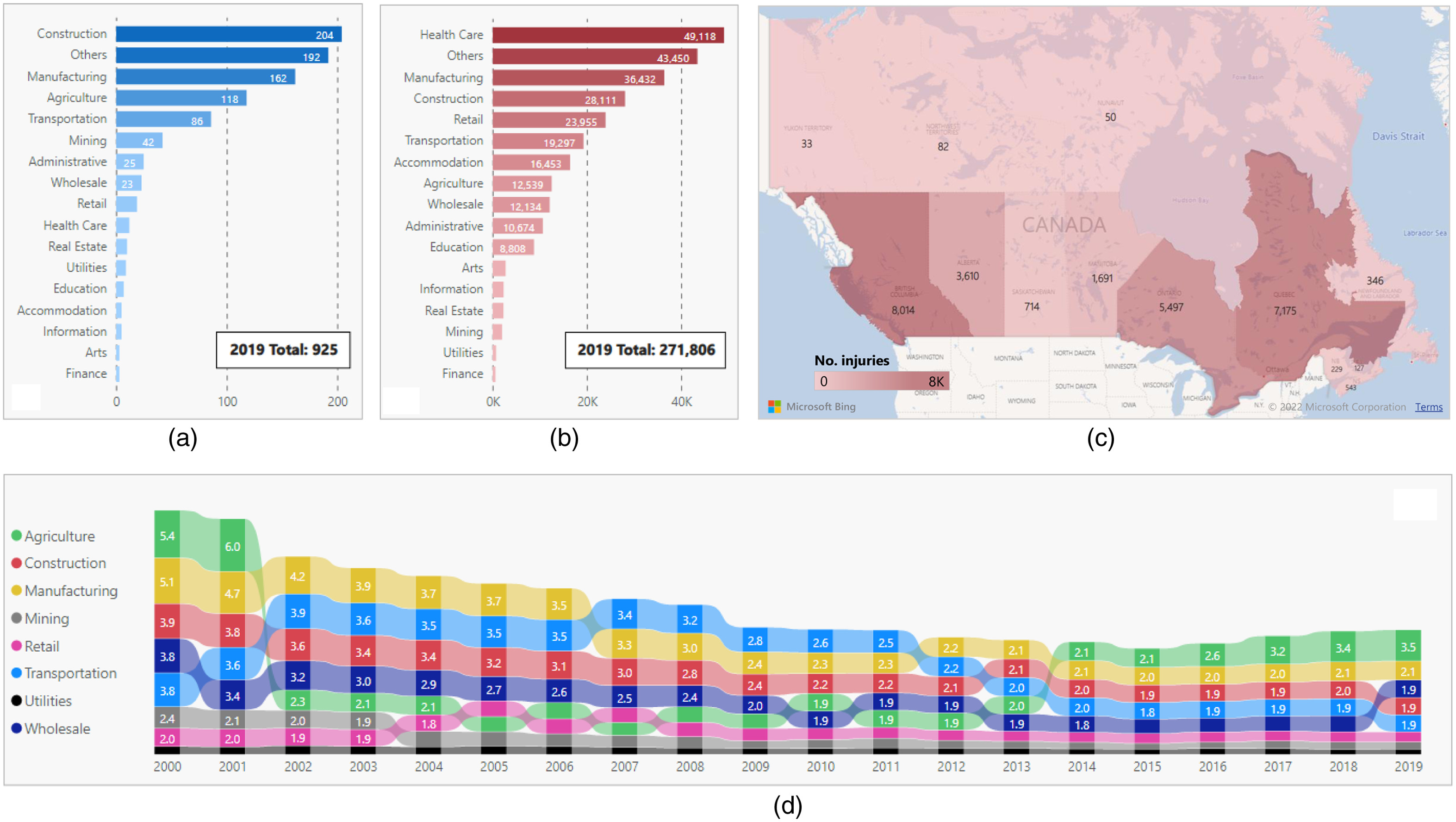
The construction industry continues to be one of the most dangerous industries worldwide (Jin et al. 2019; Marin et al. 2019; Alkaissy et al. 2020). For example, the US construction industry accounted for approximately 22% of all workplace fatalities in 2019 despite employing only about 7% of the workforce, making it the deadliest industry in the United States, with a fatality rate three times greater than the all-industry average (Hallowell et al. 2013; BEA 2021; BLS 2021a). Specifically, in 2019, the US construction industry suffered over 1,000 fatal injuries in addition to more than 200,000 nonfatal severe injuries (BLS 2021b). In Canada, the construction industry in 2019 accounted for the highest number of fatalities (204) and third highest number of severe injuries (28,111) in the workplace among all the major industries, as shown in Figs. 1(a and b), respectively (AWCBC 2021; Statistics Canada 2021). In addition, Fig. 1(c) shows all the severe injury counts in 2019 across the Canadian provinces. It can also be inferred through Fig. 1(d) that the construction industry was consistently ranked within the top three industries in Canada having the highest severe injury rates over the past two decades. Such alarming examples of fatality and injury rates, along with their corresponding societal burdens and financial losses, have elevated the urgent need for research to cultivate safer work environments across construction sites.
Primary safety research efforts have focused on identifying sets of construction injury factors (CIFs) or root causes (Zohar 1980; Dedobbeleer and Béland 1991; Mattila et al. 1994; Glendon and Litherland 2001). Such CIFs include, but are not limited to (1) project factors such as company size, project type, end use, duration, contract amount, and number of involved contractors, (2) work condition factors including worksite environment, hazard exposure, and project hazard level, (3) human factors such as human error and mental state, (4) competence factors, for example, work familiarity, site experience, and safety training, (5) production pressure factors including work pace, overload, and fatigue, (6) motivation factors including wages, incentives, and job satisfaction, (7) personal factors such as age, gender, and marital status, (8) weather factors such as temperature, humidity, wind speed, precipitation, and snowfall, and (9) safety management factors including safety programs, policies, and compliance with procedures. Recent research studies attempted to quantify the impacts of different CIFs on injury incidence; however, these studies mainly relied on opinion-based data collection methods (e.g., structured interviews and questionnaire surveys). Specifically, such studies evaluated the relative influences of the different CIFs based on professional experience and intuition of relevant safety managers (McDonald et al. 2000; Mohamed 2002; Zohar 2002; Mearns et al. 2003; Fang et al. 2006; Pereira et al. 2018). Other research studies centered around employing statistical analyses (e.g., multiple linear regression, bivariate correlation, and factor analyses) to such opinion-based collected data to study the relationships between CIFs and the incidence of injuries (Choudhry et al. 2009; Chen and Jin 2013; Marin et al. 2019; Pereira et al. 2020).
While the research efforts discussed above are certainly valuable, they have two key drawbacks. First, subjective data can, in many cases, be biased/influenced by personal/subjective judgment and “gut feeling” (Akhavian and Behzadan 2013). Second, injuries can be viewed as the outcome of combined and interdependent effects of multiple fundamental CIFs. For instance, the type of hazard exposure is typically influenced by changes to the worksite environment and/or weather conditions (Feng et al. 2014). However, to simplify the resulting statistical models, previous research efforts considered CIFs in isolation (i.e., independently), thus reducing the reliability of such models and limiting their generalization and widespread adoption (Mohammadi et al. 2018). These two drawbacks have thus highlighted the necessity for an alternative safety decision support approach, as presented in the current study.
Aligned Opportunities for a Solution
Empirical safety data and information are among the most valuable assets for organizations’ safety decision making. Currently, such digitized data and information are becoming more available as a result of legislation that requires employers from various industries, including construction, to report work-related injury and fatality incidents along with reports that describe project and worksite circumstances surrounding these incidents (Huang et al. 2018; OSHA 2021). From such reports, key CIFs and construction injury severity levels (ISLs) can be extracted and organized into database formats to facilitate their use for further analysis.
An equally important asset is a suitable data analytics platform that addresses challenges of statistical analysis techniques, as discussed earlier, to accurately extract intrinsic injury-related patterns and thus hidden safety knowledge from such empirical data sets (Zhou et al. 2019). In this context, machine learning (ML) is known to model and predict complex phenomena (e.g., construction injuries) based on interdependent variables (e.g., CIFs) and outcomes (e.g., ISL) due to its capability to discover the nonlinear complex relationships between such variables and outcomes without prior statistical assumptions (Rodriguez-Galiano et al. 2014; Siam et al. 2019; Gondia et al. 2020).
ML predictive modeling has gained increasing attention in construction safety research in recent years, and has been applied to predict the likelihood of incident types (Tixier et al. 2016; Gerassis et al. 2017; Kang and Ryu 2019; Ayhan and Tokdemir 2020) and incident risk levels (Zhou et al. 2017; Poh et al. 2018; Sakhakarmi et al. 2019), and to assess construction safety climate scores across projects (Patel and Jha 2015; Abubakar et al. 2018; Makki and Mosly 2021). However, most models developed in such research works are essentially “black boxes” (e.g., random forests, artificial neural networks, and support vector machines) that would hinder interpretation of the underlying causation and interrelationships between CIFs and ISL, thus ultimately limiting qualitative safety judgment (Li et al. 2012; Kakhki et al. 2019). In this regard, discussions are emerging in construction safety prediction research about “glass-box” ML methods, which not only enable quantitative predictions but also support qualitative judgement through transparent insights that can also deepen managers’ understanding of the cause-and-effect relationships between CIFs and ISL. For example, decision tree (DT) models are among the few powerful glass-box/transparent ML models that can explicitly link/map combinations of CIFs to different outcomes of ISL through rules. These rules can also be used to predict the most likely outcomes for new construction site circumstances (Chi et al. 2012). Random forests (RFs), on the other hand, adopt an ensemble of DTs and aggregate their predictions, which improves the overall predictive performance of the models but again limits their interpretability (Kuhn and Johnson 2013). Moreover, it remains unclear in construction safety prediction research the extent to which glass-box models are comparable to black-box counterparts in terms of predictive accuracy—a discussion that can facilitate rationale for transparency/performance tradeoff and model selection criteria.
Goal and Objectives
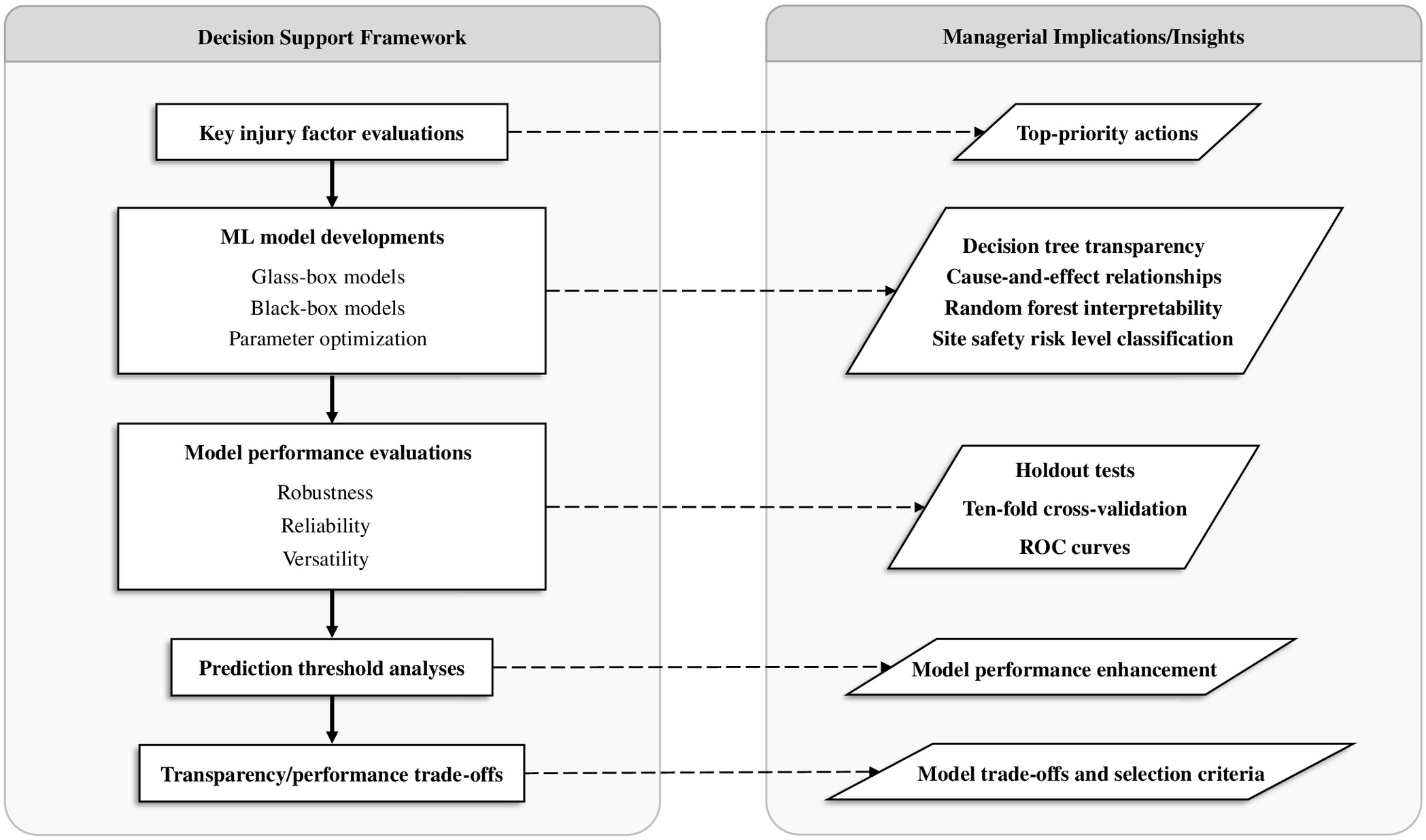
Adopting specific ML models, the current study developed an empirical data-driven construction safety decision support framework (Fig. 2) that enables quantitative construction injury prediction while also supporting qualitative safety judgment and interpretation. As shown in Fig. 2, key injury factors were initially evaluated and identified, upon which top-priority safety decisions can be based. Subsequently, glass-box and black-box ML models (where DT and RF models are adopted as respective possible candidates herein) were developed to facilitate predicting ISL from the interdependent effects of CIFs, upon which better-informed and transparent and/or interpretable safety decisions can be based. All model developments considered the key step of parameter optimization to yield unbiased/generalizable models. The predictive performance of the developed models was further verified using cross-validation tests and multiple relevant performance evaluation measures. In this respect, receiver operating characteristics insights were provided to support decision making in adjusting model prediction thresholds to enhance the overall model performance. Finally, decision support on model selection was provided based on a tradeoff between DTs’ transparency and RFs’ expected higher performance. To demonstrate the framework utility and show examples of key extractable learnings/managerial insights, an Occupational Safety and Health Administration construction site injury case data set was used. Employing the developed framework, safety managers can evaluate different construction sites’ safety risk levels and classify them, based on predicted injury severity and probability levels, as high-risk or low-risk zones for ultimately formulating and disseminating prevention strategies in a more targeted and proactive manner.
Framework Architecture
Key Injury Factor Evaluations
CIF evaluation and ranking can be performed on empirical injury case data sets to (1) quantitatively evaluate the relative importance of CIF contributions to ISL, (2) identify key CIFs with the greatest influence on ISL to use for making top-priority safety decisions, and (3) proceed with such key CIFs to create a simplified data set that would reduce computation time and increase subsequent ML model accuracy (Gerassis et al. 2017; Zhang et al. 2020). The information gain attribute evaluator (IGAE) was used as the variable evaluation algorithm in the current framework due to its known accuracy with categorical variables and its ability to learn potentially disjunctive patterns (Chi et al. 2012; Aggarwal 2015). The IGAE is based on information-theoretic measures of entropy and gain that are calculated for each variable (i.e., CIF) in the data set (Shannon 1948). Generally, information entropy () is a measure of uncertainty in a variable and denotes the lack of predictability from that variable, whereas information gain () is inversely proportional to entropy and infers the amount of information added to the prediction process by including such a variable. For example, variables with lower values (i.e., higher values) are more significant within the data set. Given a variable with a distribution of , the of the variable is computed as given in Eq. (1) (Wang et al. 2010; Aggarwal 2015). The greater the variable distribution randomness, the less the variable contains, which indicates that the maximum (i.e., least conveyed information) is observed when the variable is uniformly distributed
(1)
When applying the IGAE to a data set that contains multiple CIFs, each with varying numbers of categories/values, and an outcome ISL with several underlying classes, Eqs. (2)–(4) are adopted to calculate class-based entropy (Aggarwal 2015; Gerassis et al. 2017; Zhang et al. 2020). First, the base entropy, , is calculated for the entire data set using Eq. (2), which is based on the counts of each class within the data set. This is followed by computing the conditional entropy, , for each category within every CIF using Eq. (3). The latter is the weighted summation of entropies pertaining to a category’s distribution across the two classes. The weighted average entropy, , over all categories within each CIF is then calculated for each CIF, as shown in Eq. (4). CIFs with higher imply a greater mixing of the two classes with relation to the distributions of the categories, while a CIF with an value of zero implies perfect separation and, therefore, the greatest possible predictive power. The final step is to compute values of information gain, , for each CIF. The gain in information due to a specific CIF is the difference between the information conveyed for predicting the ISL from the data set before and after the introduction of that CIF. Specifically, the of the th CIF is the difference between the base entropy of the data set and the weighted average entropy of that CIF, as demonstrated in Eq. (5). Therefore, information gain indicates a reduction in entropy, and the most informative/influential CIF toward ISL is that with the highest where = total number of classes; = class; = total number of cases in the data set; = number of cases of the th class; = variable or CIF; = category; = number of cases of the th category within the th variable belonging to the th class; = total number of cases of the th category within the th variable; and = total number of categories within the th variable.
(2)
(3)
(4)
(5)
ML Model Developments
The injury cases data set is split into a training set (e.g., 80%) and a testing set (e.g., 20%). The training set is used to train/develop the ML models and the testing set is later introduced to evaluate the predictive performance of such models.
Glass-Box Models
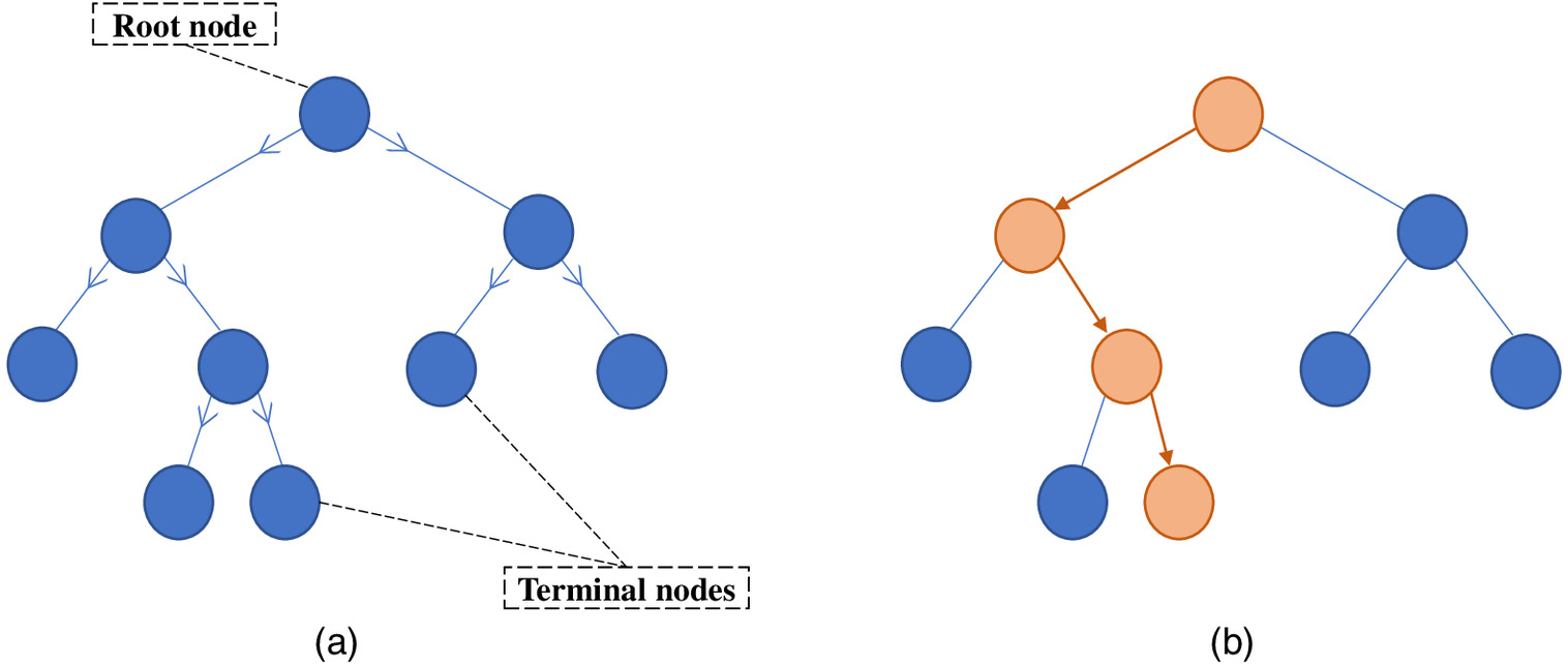
In the current framework, DT models were adopted as candidates of glass-box models. Specifically, three different and commonly used DT models were applied: recursive partitioning and regression trees (RPART) (Therneau and Atkinson 2018); classification and regression trees (CART) (Ripley 2018); and C4.5 (Hornik et al. 2009) models. By comparing the performance of these three models, their validity can be further tested, and the most appropriate model for construction injury prediction can be identified. Generally, DT models are based on the recursive splitting of the data cases into subsets represented as nodes, where such nodes expand to form a top-down tree-shaped structure [Fig. 3(a)] that describes the decision (and thus prediction) flow (Breiman et al. 1984; Chi et al. 2012; Gondia et al. 2019). Starting from the root (i.e., top) node, the IGAE procedure described earlier is applied on the data subset comprising each node, and the most predictive CIF (i.e., most influential toward ISL) is then selected for splitting such node through two branches into two child nodes. The CIF categories are selected across the branches in a way that maximizes the class homogeneity of the resulting child nodes (i.e., yields the cleanest split in terms of the ISL class). Such node splitting is repeated until all cases within a node belong to only one of the ISL classes, marking a perfect classification and designating such node as a terminal node. Once all terminal nodes are reached, the splitting process concludes, and the resulting final tree can be used for predicting the classes of new cases. As a glass-box ML model, DT facilitates such prediction through an explicit/transparent mapping of CIF combinations and corresponding categories to an ISL class by descending from the root node until reaching a terminal node, as shown in Fig. 3(b).
If a DT model is allowed to grow indefinitely until all terminal nodes are reached, the resulting tree may become extremely complex due to its numerous nodes. Not only will a complex tree complicate its interpretability, but also such a tree will have learned the unique peculiarities of the training set rather than its general structure, causing the tree to be incapable of generalizing to new cases—an issue known as overfitting (Kuhn and Johnson 2013). Therefore, tree pruning, through “snipping off” the least important splits, can avoid overfitting. A key step to such tree pruning is optimizing the tree parameters that control tree complexity. In this respect, the objective of tree parameter optimization is to find the optimal level of tree complexity that achieves the right tradeoff between predictive accuracy on that training set and another set of new data (Bergstra and Bengio 2012). In this regard, the DT models demonstrated later in the current study were developed through a generalizable approach by tree parameter optimization, where a tenfold cross-validation procedure is applied repeatedly to the training set only, with nine training folds and a single alternating validation fold (Arlot and Celisse 2010). For each tenfold cross-validation procedure, a specific tree parameter value was selected and the average predictive error (i.e., 1-accuracy) of the resulting trees over the 10 validation folds was recorded. Several procedures were repeated to search through the parameter space, and parameters achieving the minimum average cross-validation error were selected to yield the optimal model.
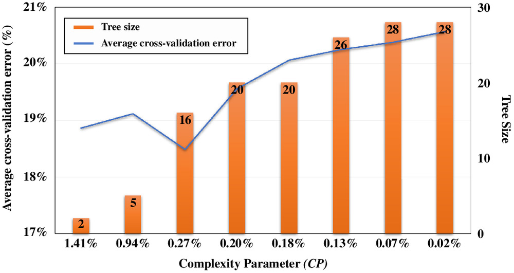
For the RPART model, the parameter to be optimized is the complexity parameter (CP), which is the minimum improvement in model accuracy needed for a node to be allowed to split. Specifically, while growing the tree, a split is not pursued if it does not minimize the model’s predictive error by a factor of CP. Regarding the CART model, the parameter available to be optimized is the maxdepth, which refers to the maximum tree depth in which the tree is prevented from growing past that depth. The depth of a tree is the length of the shortest path from a root node to the deepest terminal node where, for example, the tree in Fig. 3(a) has a depth of three. For the C4.5 model, the parameter that needs to be optimized is the minsplit, which refers to the smallest number of cases inside a node that could be further split. If a node comprises a number of cases less than the set minsplit value, it is labeled as a terminal node and does not continue to grow.
Black-Box Models
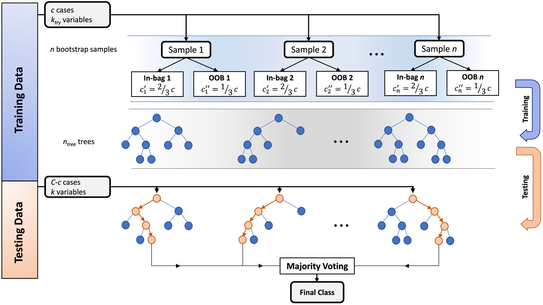
Adopted as black-box model candidates herein, RF models are also tree-based models that involve growing/training many single DTs to form a forest that predicts new cases by combining the output of each tree (Breiman 2001; Zhou et al. 2019). This combination yields an RF model that can typically achieve better predictive performance than any one individual DT (Rodriguez-Galiano et al. 2012). More precisely, for a data set with a total of cases (of which are training cases) and variables (i.e., CIFs), the RF procedure is implemented as illustrated in Fig. 4. First, a number of data samples (each of the same size as the training set) is created using bootstrap random sampling with replacement from the original training set, which means that some cases may be repeated (within the same sample) or left out. Two-thirds of the cases are randomly designated as in-bag cases and are used for tree training, while the remaining one-third is left out for parameter optimization (discussed next) and is known as the out-of-bag (OOB) set. Second, each in-bag set is used to build a corresponding decision tree; however, at each node of the tree, a subset of variables (which is not greater than the total number of variables) is randomly selected, and the best predictive variable from that subset is used for node splitting. Third, each tree contributes with a single vote of a predicted class to the forest, and the final prediction result is obtained by considering the majority vote (i.e., the class with the higher frequency of votes). Overall, randomizing the sampling procedure and only trying a random subset of variables at each split result in dissimilar trees (as each is grown on a different data sample and variable subset) with reduced correlations, which ultimately improves the RF model generalization performance. A similar ML technique, bootstrap aggregating (bagging) has one (but key) difference from RF in that the former considers all variables at a node for splitting. This produces single trees that are highly correlated when subjected to a data set having variables that are strong predictors (Breiman 1996; Han et al. 2018). However, combining the results of single trees that are essentially similar/correlated does not typically lead to large improvements in generalizability (Zhou et al. 2019), the effects of which will be evaluated in the application demonstration.
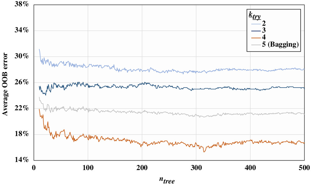
Two major RF parameters need to be optimized, namely the number of trees in the forest (i.e., same as the number of obtained bootstrap samples) and the number of variables randomly considered at each node split. An value that is too small may result in insufficient training, and a value that is too small may lead to underfitting. In contrast, and values that are too large may cause both overfitting and prolonged computation time. Therefore, different combinations of these two parameters were used in the current study to sequentially train RF models on the in-bag set (Fig. 4). This training is followed by introducing such resulting models to the OOB set (presenting new data that were not used in training) to calculate the average OOB error. The parameter combination resulting in the lowest average OOB error is the optimal one.
Model Performance Evaluations
To evaluate the performance of the ML predictive models considered within the framework, confusion matrices (Chou and Lin 2013; Seong et al. 2018) are primarily produced. As presented in Table 1, such a confusion matrix exhibits numbers of predicted and actual ISL classes, where the diagonal represents correct predictions and the off-diagonal represents incorrect predictions. For demonstration, the example in Table 1 assumes two ISL classes, fatal and nonfatal injuries. From such confusion matrices, several performance evaluation measures are then derived. Accuracy evaluates the overall performance of a model and describes the percentage of correct predictions relative to the total number of predictions [Eq. (6)]. As it is particularly important to evaluate the model’s ability to accurately predict fatalities, precision measures how many of the predicted fatal cases are correct. However, the implication of overlooking a fatality by predicting it as a nonfatality (FN) is more serious than incorrectly predicting a nonfatality as a fatality (FP). Accordingly, true positive rate (TPR) is also a suitable measure to consider because it takes FN into account [Eq. (8)], unlike precision. Finally, true negative rate (TNR) describes the percentage of correctly predicted nonfatalities relative to the total number of actual nonfatalities [Eq. (9)]
(6)
(7)
(8)
(9)
| Actual class | Predicted class | |
|---|---|---|
| Fatal | Nonfatal | |
| Fatal | True positives (TP) | False negatives (FN) |
| Nonfatal | False positives (FP) | True negatives (TN) |
Such measures enable the evaluation of the robustness, reliability, and versatility of the developed model’s prediction, as presented next.
Robustness
Model prediction robustness can be evaluated using holdout testing, where the entire data set is split into 80% training set and 20% testing set. The splitting is carried out in a stratified manner, where both training and testing sets have similar distributions of the ISL classes (Kohavi 1995; Fiore et al. 2016). The former set is used to train the models, while the latter set is used to present the trained model with essentially new data to test its predictive robustness through the confusion matrix and multiple evaluation measures, as discussed earlier.
Reliability
Evaluating a model’s prediction reliability can be carried out through k-fold cross-validation, where the entire data set is divided into separate and almost equally sized folds in a stratified manner with regard to the ISL classes. folds are combined for training and the remaining fold is set aside for testing. Such training and testing are then repeated times, such that each of the -folds is used exactly once for testing. For each test fold, a confusion matrix is generated, and a corresponding set of evaluation measures is derived and subsequently averaged over the -folds. Compared to the holdout testing method, the main advantage of -fold cross-validation is that the entire data set is utilized in training and the testing procedure is carried out times, thus allowing a better evaluation of the generalization capability of the developed model. This allows for an assessment of the model’s reliability when applied repeatedly to several unseen future data sets.
Versatility
A model’s prediction versatility can be evaluated through the inspection of its receiver operating characteristic (ROC) curve and the area under that curve (AUC). Such an approach is also useful in applications where the impact seriousness of two prediction errors is significantly unequal (i.e., FP and FN) (Son et al. 2014). Typically, the final prediction of an ML model is based on the highest predicted probability of the available classes, and thus for a prediction problem with two classes, the default prediction threshold is 0.5. In this regard, the receiver operating characteristic space is presented by a 2D graph, where values of TPR are plotted on the -axis and values of false positive rate (FPR) (where ) are plotted on the -axis for multiple prediction thresholds ranging from 0 to 1. A model with a larger AUC indicates better versatility in predictive performance because this implies that a larger value of TPR can be achieved for each value of FPR across many different thresholds. Therefore, the AUC evaluates the versatility of the model’s predictions irrespective of what threshold is used.
Prediction Threshold Analyses
As described earlier, instead of considering only the default prediction threshold of 0.5, the ROC curve follows the process of (1) varying the threshold values in the range between 0 and 1, (2) storing the corresponding designations of actual and predicted ISL classes for each threshold value, (3) producing corresponding confusion matrices, and (4) plotting corresponding combinations of TPR and FPR. The ROC curve thus provides a visual tool to better understand the predictive performance of the model on a wide range of thresholds. Such curves demonstrate the tradeoffs pertaining to increasing the model’s probability of incorrectly designating a nonfatality as a fatality (i.e., FPR) for ultimately improving its probability of successfully detecting fatalities (i.e., TPR). Safety managers can use such a tool to adjust their model with a better threshold selection and obtain a more suitable combination of FPR and TPR probabilities that meet the specific needs of each construction site, as we will present in the demonstration application.
ML Transparency and Interpretability
ML interpretability can be categorized into two groups, model-specific or model-agnostic (Molnar 2020). Model-specific interpretability is limited to particular models (e.g., linear regression, logistic regression, DT, and genetic programming-based models), which are inherently glass-box transparent models because their internal structure follows an explicit mathematical or rule-based expression (Naser 2021), as will be discussed later in the context of DT. Other ML models (e.g., RF), however, might not reveal such explicit input–output relationships/sensitivities, which is why such models are commonly referred to as black-box models. In this context, model-agnostic interpretability has become a very popular research point recently to demystify the long-criticized black-box nature of some ML models, through supporting users of such models with insights about (1) the cause of model decisions (i.e., the outcome for given inputs), (2) the variables that are the most important to the model, or (3) the model outcome variations due to changing one or more selected variables (Feng et al. 2021). As their name suggests, model-agnostic methods are not model-dependent and can be used across different models (e.g., RF) because they are typically applied in postmodel training. Examples of such methods are described as follows:
•
Variable importance algorithms can improve a model’s interpretability by understanding the influence/importance of its variables (e.g., CIF) toward the prediction process (e.g., ISL prediction). Such algorithms measure/quantify the extent to which a model relies on a particular variable by evaluating the model’s increase in prediction error or change in prediction entropy after permuting such variable, where the relative importance of that variable is based on the corresponding relative increase in model error or entropy (Altmann et al. 2010; James et al. 2013).
•
SHapley Additive exPlanations (SHAP) algorithms (Lundberg and Lee 2017) not only provide variable/CIF importance in an average sense, but also quantitatively explain how each variable affects the model’s predictions for the whole data set (i.e., global interpretation) and for a given individual data point/injury case (i.e., local interpretation) (Štrumbelj and Kononenko 2014; Lundberg et al. 2020).
•
Partial dependence plots (PDP) (Goldstein et al. 2015) depict the marginal effect of an individual (or group of) variable/CIF on the model’s ISL predictions while holding other variables constant within the same model, and can also be used to infer the type of relationship between variables and outcomes (e.g., whether linear, nonlinear, or complex). When applied to classification problems, this method gives the probability for a particular class due to varying variable values (Friedman 2001).
•
Surrogate models (Nyshadham et al. 2019) use an external secondary model, which is typically more implicitly interpretable (e.g., linear models, genetic algorithms, tree-based models), to simplify the explanation of the considered model’s predictions. These surrogate methods are employed to capture the predictions of the original model given the set of input variables/CIFs, thus providing insights into why the complex model predicts the way it does in a more explainable way (Gorissen et al. 2010).
Model Transparency/Performance Tradeoffs
While DT models offer valuable glass-box transparency merits, RF (black-box) models may offer better predictive performance improvements, albeit with restricted interpretability, which can then be enhanced using model-agnostic methods as discussed above. To that end, this subsection can provide analysts with the criteria for which model to select under different characteristics of the injury cases data at hand. First, RF models are more robust to unbalanced distributions of the outcome class compared with individual DT models (Zhou et al. 2016; Hong et al. 2017). Second, RF models can better handle data with large numbers of input variables (Abdel-Rahman et al. 2013; Liu et al. 2018). Third, RF models may perform better than single DTs on data with strong predictor variables alongside other potentially irrelevant variables (Sutton 2005; James et al. 2013), as discussed earlier. The application presented next will further demonstrate how managers can use this decision support to assess the tradeoff between transparency and performance according to their unique application requirements and data characteristics.
Demonstration Application
Data Set Description and Visualization
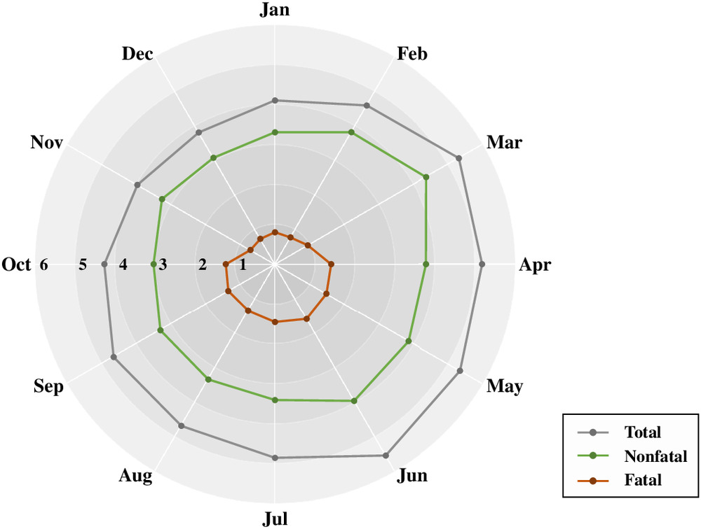
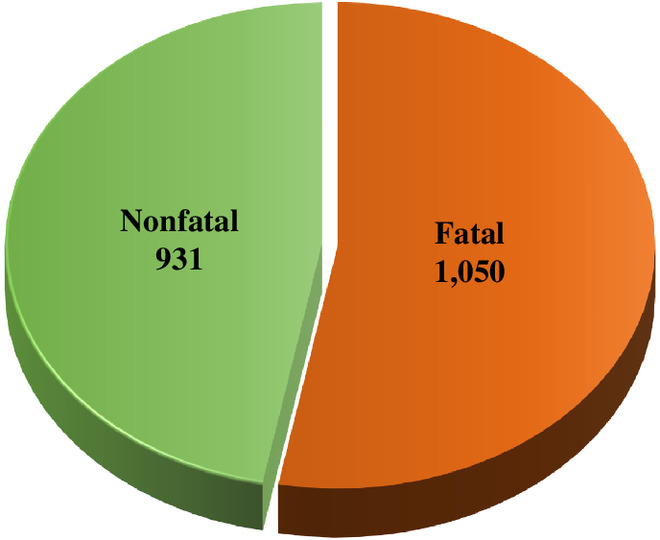
The data set used in the current demonstration was obtained from the Occupational Safety and Health Administration (OSHA) injury cases data set (OSHA 2019) where, at the time of access, approximately 3,400 cases corresponded to US construction projects. These cases contained CIF information describing the work circumstances at the time of the injury and the outcome ISL, whether fatal or nonfatal. Fig. 5 shows the average number of injuries per day for each month. As can be seen in the figure, more injuries occurred during nonwinter months (e.g., May and June) than in winter months (e.g., December and January), because more construction activities are typically executed during warmer weather. Eight CIFs were provided: (1) project type, (2) project end use, (3) contract amount, (4) worksite environment, (5) hazard exposure, (6) human error, (7) work familiarity, and (8) month. However, many of the nonfatal injury cases contained missing CIF-related information. Therefore, such cases were not considered in the current study, thus reducing the data set to a total of 1,981 injury cases with a complete set of eight CIFs and one corresponding outcome ISL (1,050 fatal and 931 nonfatal). This preprocessing step was necessary to convert the remaining cases into a readable data set to enable the subsequent ML analysis.
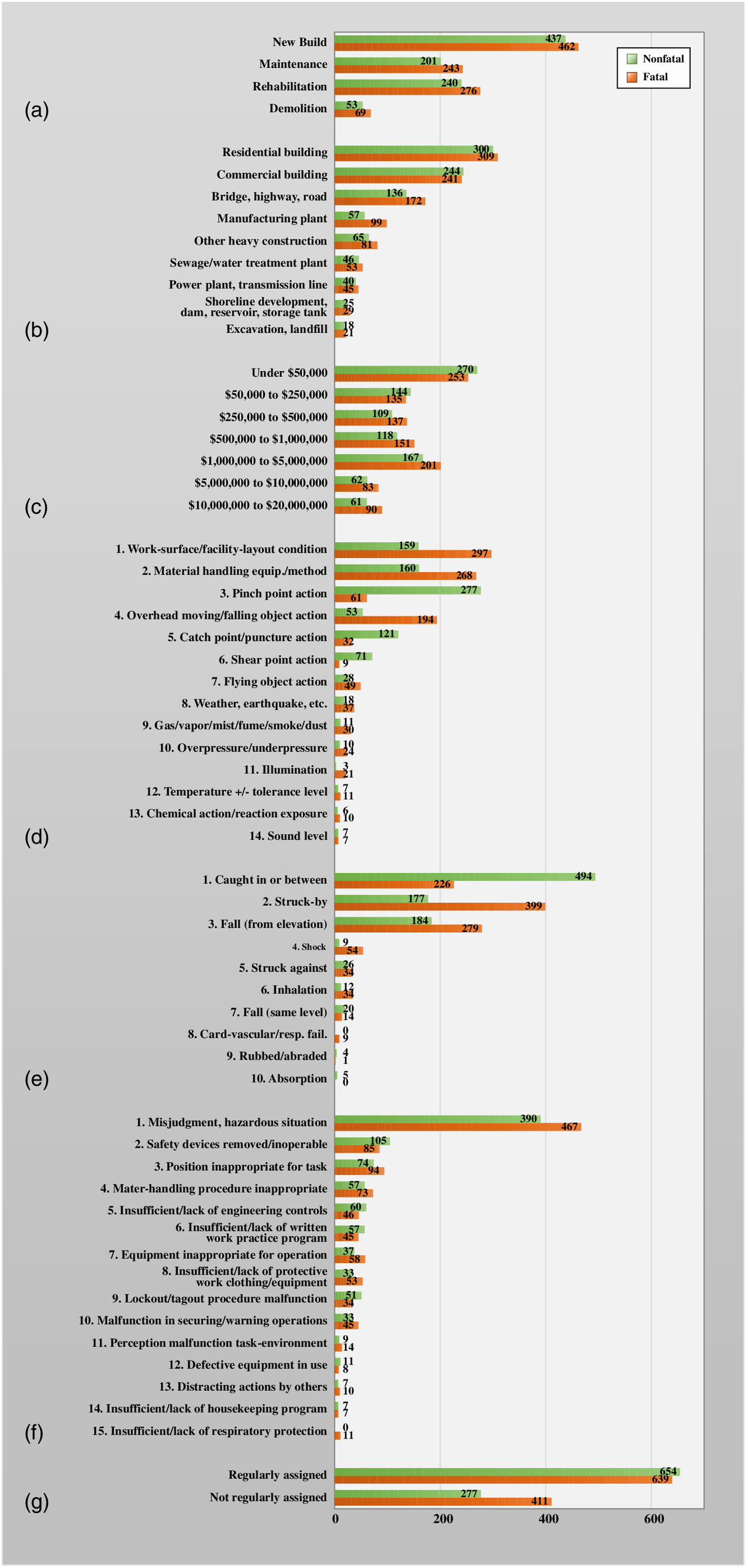
Within the reduced data set, the distribution of categories of project type, project end use and contract amount across ISL classes are shown in Figs. 6(a–c), respectively. Worksite environment denotes the unsafe nature of the working conditions surrounding or in close proximity to the worker, while hazard exposure is related to the dangers associated with the specific task performed by the worker at the time of the injury. The category distributions of these two CIFs are presented in Figs. 6(d and e), respectively. In addition, the category distributions of human error, work familiarity, and ISL are shown in Figs. 6(f and g) and 7, respectively. As there were no spatial data included in the data set to match the date for deriving weather data, the month was considered as a CIF to represent weather factors. It can be seen from these figures that, although some CIFs have visible effects (i.e., clear distinctions) on ISL outcomes [e.g., worksite environment in Fig. 6(d) and hazard exposure in Fig. 6(e)], other CIFs have less significant effects (i.e., balanced distributions) on ISL [e.g., project type in Fig. 6(a)]. This finding suggests that different CIFs might have varying influences on ISL and, thus, varying significance toward the prediction procedure, which underlines the need for a CIF importance quantitative ranking.
Top-Priority Actions
The IGAE presented in Eqs. (2)–(5) was applied to the data set, where ; or 2 (i.e., 1 = fatal and 2 = nonfatal); ; or (i.e., and ); to 8 (e.g., 1 = project type, 2 = project end use, etc.); is the category for each CIF (e.g., for project type, 1 = new build, 2 = maintenance, etc.), and is the total number of categories within the th CIF (e.g., 14 for worksite environment). The information gain results are shown in Fig. 8. The top three ranked CIFs according to their corresponding values are month (0.356), worksite environment (0.317), and hazard exposure (0.302). This finding is supported by the visualizations presented earlier, where the category distributions of such CIFs over the two ISL classes had visible separations in Figs. 5 and 6(d and e), respectively. The fourth and fifth CIFs are human error (0.165) and work familiarity (0.101), which is also apparent from more balanced distributions of such CIF categories over the two ISL classes in Figs. 6(f and g), respectively. The lowest-ranked CIFs are project end use (0.016), contract amount (0.011), and project type (0.007), indicating that these CIFs have the least effect on ISL.
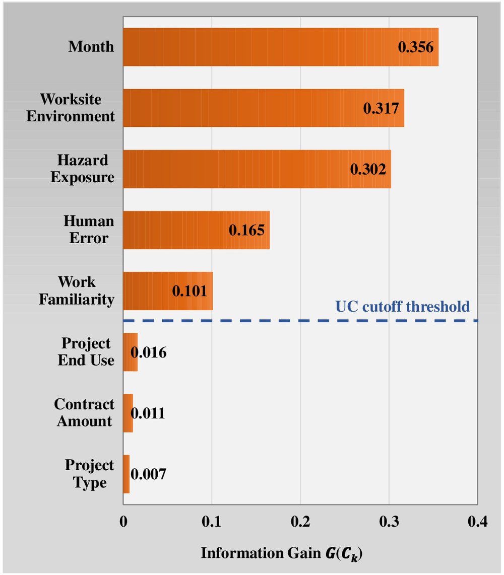
In selecting the key CIFs to proceed with, the average uncertainty coefficient (UC) is used as a cutoff threshold to exclude irrelevant CIFs (Desai and Joshi 2010). The UC for each CIF is calculated as the ratio of to , and then the CIFs with a UC value greater than the average UC value are selected to proceed with during the subsequent ML analyses. Based on the UC values (Fig. 8), the top five CIFs are considered to be key CIFs, namely month, worksite environment, hazard exposure, human error, and work familiarity, whereas the bottom three CIFs are excluded from the data set, which are project end use, contract amount, and project type. This selection also aligns with several previous studies (Cooper and Phillips 2004; Behm 2005; Choudhry et al. 2009), which highlighted that project-related factors and personal demographics (e.g., the bottom three CIFs) have less significant relationships with injury outcomes compared with safety-related factors and site situational conditions (e.g., the top five CIFs).
Injury prevention begins with having a clear understanding of the CIFs that significantly influence safety in construction projects. In this regard, the described IGAE procedure can help managers pinpoint those key CIFs to better invest in injury prevention and risk mitigation strategies that are of top priority. This procedure can be useful as a decision support tool in the planning stage of the construction project, especially when a large number of CIFs must be considered. In the current application, for example, the procedure pointed to weather factors, worksite environment, and hazard exposure as the CIFs that need the greatest attention. Such actionable feedback can guide managers, from the onset, in developing prevention strategies that mitigate risks pertaining to the following: (1) weather conditions, through appropriate personal protective equipment regulations, emergency weather evacuation planning, and relevant weather safety training, (2) worksite environment, by preparing practical site-specific safety plans, conducting hazardous conditions inspections, and equipping workers with knowledge about physical protection in complicated sites and working from heights, and (3) hazard exposure, through job hazard analyses, pretask safety planning meetings to ensure that hazards are recognized and communicated prior to worker exposure, safety programs for operating equipment, regular equipment maintenance, and emergency response drills.
Model Developments
As previously described, the data set (1,981 cases) was split, with 80% forming a training set (1,585 cases) and 20% forming a testing set (396 cases). The DT models were developed through a generalizable approach using tree parameter optimization through a tenfold cross-validation procedure applied to the training set. The results for the RPART model are shown in Fig. 9, where, as previously discussed, higher values of CP are more likely to restrict tree growth, while lower values of CP are more lenient to node splitting and result in larger tree sizes (i.e., number of terminal nodes). As shown in the figure, a CP value of 1.41% results in the smallest tree size of one split into two terminal nodes, while a CP value of 0.02% allows all splits and thus produces the largest tree possible with a tree size of 28. From the figure, the optimal CP value for the current RPART model is 0.27%, resulting in a minimum average cross-validation error of 18.49% and tree size of 16. Also based on the tenfold cross-validation results, the maxdepth for the current CART model is limited to an optimal value of five, which corresponds to a minimum average cross-validation error of 19.24%. Furthermore, the optimum minsplit value for the current C4.5 model is 15, resulting in a minimum average cross-validation error of 19.75%.
The RF model parameters are optimized based on the average OOB error. As shown in Fig. 10, the range of is set from 5 to 500 with a step size of 1, and values of between 2 and 4 (i.e., RF) as well as all 5 (i.e., bagging) variables are also considered—which means that 1,980 iterations of successive parameter combinations, and thus RF models, are evaluated. Based on the results, the optimal combination of parameters is and , resulting in a minimum average OOB error of 15.31%. The figure also shows that using a value of all five variables does not provide the least average OOB error, which confirms the need for RF over bagging to inject more randomness in each bootstrap sample, thus producing less correlated trees and a more generalizable model.
Model Performance Evaluations
Holdout Tests
Using the aforementioned optimal parameters for training, the results of the holdout testing for the four models are reported in Table 2. The table includes performance evaluation measures of accuracy, precision, TPR, FPR, and the average of such measures to establish an overall score for each model. Generally, the four models perform well as the average score of each model is always higher than 80%, which also confirms the reliability of the selected CIFs. Based on the measures in the table, the CART and C4.5 models demonstrate comparable performances, with the former slightly outperforming the latter with respect to the average score. However, the RPART model is the best-performing DT model in every measure including accuracy (81.82%), precision (81.08%), TPR (85.71%), TNR (77.42%) and thus average score (81.51%). As discussed, TPR is especially observed as the predictive performance of the fatal class is particularly important. The RPART model performs well, leaving only a 14.29% chance that a fatality will be mispredicted as a nonfatality. Regarding the RF model, the results of the holdout testing in Table 2 indicate that this model outperforms its singular DT model counterparts, including the RPART model, in terms of all the performance evaluation measures as accuracy (83.84%), precision (82.59%), TPR (88.10%), and TNR (79.03%), attaining an average score of 83.39%.
| Model | Accuracy (%) | Precision (%) | TPR (%) | TNR (%) | Average score (%) |
|---|---|---|---|---|---|
| RPART | 81.82 | 81.08 | 85.71 | 77.42 | 81.51 |
| CART | 80.56 | 80.09 | 84.29 | 76.34 | 80.32 |
| C4.5 | 80.30 | 80.28 | 83.33 | 76.88 | 80.20 |
| RF | 83.84 | 82.59 | 88.10 | 79.03 | 83.39 |
Tenfold Cross-Validation
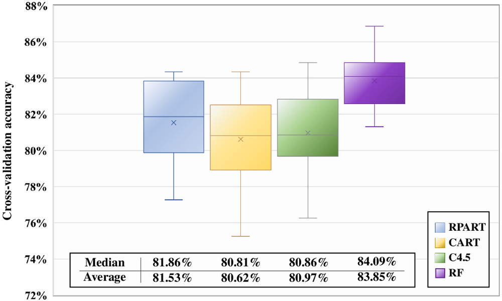
Fig. 11 demonstrates the results of a tenfold cross-validation as box plots representing the maximum, minimum, interquartile range, median, and average of the 10 resulting accuracy values. Compared to the CART and C4.5 models, the RPART model’s higher median (81.86%) and average (81.53%) accuracy indicate its better generalization capability among the tree models. In addition, the RF model’s better cross-validation performance is demonstrated through its (1) highest median and average accuracies of 84.09% and 83.85%, respectively, (2) highest maximum and minimum recorded accuracies, which are included between 86.87% and 81.31%, respectively, and (3) smallest max–min range over 10 testing folds of 5.56%, which remains more stable than the ranges pertaining to singular trees (e.g., 7.07% of the RPART model). The latter finding confirms that the RF model not only generalizes better to unseen data but can also achieve consistent performance (i.e., it is more reliable) over multiple new data sets.
ROC Curves
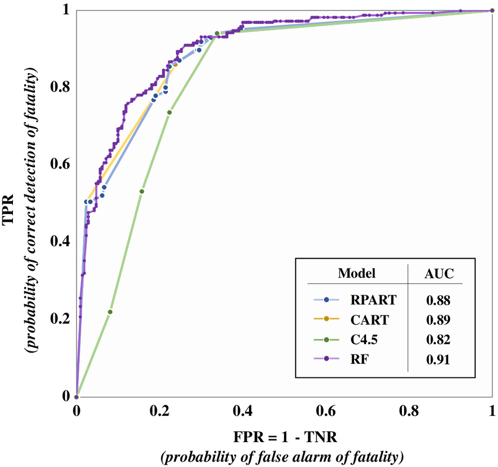
The receiver operating characteristic curves for the four models are presented in Fig. 12. The figure shows that the curve for the RF model lies above the rest which, supported by the highest quantified AUC value of 0.91, speaks to the versatility of the RF model under different prediction thresholds, and further underlines its ability to avoid serious types of prediction errors (i.e., FNs).
Model Comparisons and Tradeoffs
As can be seen from the results discussed above, while the RF model achieves higher performance, it does not significantly outperform its DT counterparts. For instance, the RF model outperforms the RPART model by only 2.02% in accuracy, 2.39% in TPR, and 0.03 in AUC. In that context, within the current construction safety and injury prediction application, DT models can be recommended for use because they (1) preserve good predictive performance, (2) provide valuable glass-box transparency-related merits (discussed next), and (3) require shorter computation times, which is conducive to rapid decision making.
The reasons behind this observed performance similarity can be considered within the context of the three criteria/rationale discussed earlier. The first criterion is related to RF models being more robust to unbalanced distributions of the outcome class. Within the current application, the outcome ISL had a relatively balanced distribution (Fig. 7), which is why the RF model did not exhibit largely superior performance over its tree counterparts. Nonetheless, in other situations, managers may consider RF modeling. The second criterion is related to how RF models can better handle data with large numbers of input variables. For example, if the injury cases data set used herein had contained a large number of CIFs describing more features of the work circumstances at the time of the injury, an RF model may be considered. The third criterion relates to how RF models may perform better than single trees on data with strong predictor variables alongside other potentially weak variables. In applications where CIFs selection is not performed (unlike the current application), there may be large differences in the influences of different CIFs on the ISL (e.g., see Fig. 8), and managers may consider RF modeling in such cases. Despite the closeness in performance between the RPART and RF models within the current application, the gap between the model performances may widen under different safety applications, and an RF model may be more suitable in scenarios where considerable improvements in predictive performance can be achieved.
Decision Tree Model Transparency
Fig. 13 shows the developed RPART decision tree model, which was selected for demonstration because it is the best-performing single tree model in the current study. The tree has a depth of 8 and contains 16 terminal nodes that indicate the predicted ISL class as fatal or nonfatal. Because the tree is earlier pruned to achieve better generalizability, the terminal nodes quantify the probabilities of each ISL, rather than providing perfect classifications, and the outcome ISL designation follows the more probable one (i.e., the default prediction threshold is 0.5, as discussed earlier). The tree branches comprise a series of logical decisions, where each branch indicates one of the five key CIFs (i.e., month, worksite environment, hazard exposure, human error, or work familiarity) and corresponding categories. Some categories are referenced through numbering consistent with Figs. 6(d–f) to keep the tree aesthetic and size efficient. Because the IGAE is applied at each node to select CIFs for node splitting, the higher branches of the tree contain the more influential CIFs, as recorded in Fig. 8.
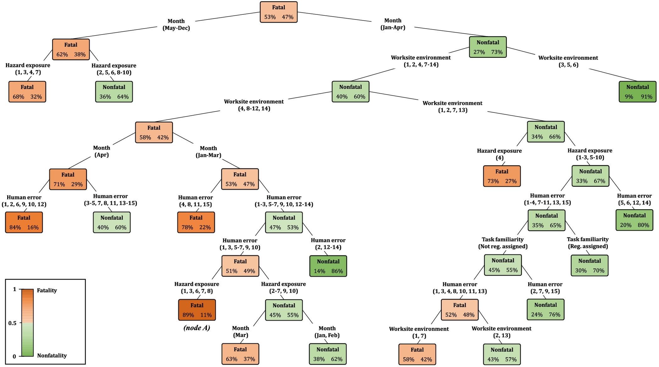
Such a glass-box model provides a transparent decision flow structure that can empower safety managers with the ability to qualitatively explore intercausal reasoning within the construction injury phenomenon. The tree establishes explicit cause-and-effect relationships by mapping combinations of CIFs (causers) to an ISL (effect), which managers can use to evaluate the interrelatedness among certain CIF categories and their combined contributions toward ISL. For example, one can elaborate by isolating the most risk-prone terminal node in Fig. 13, which is the sixth terminal node from the left, marked as node A. The results of the following combinations of CIF categories leading to this node infer that, in US construction sites, work during the winter months (January to April) typically leads to worksite environments with difficult weather conditions [e.g., (12) temperature ± tolerance level; (10) over/underpressure; (9) gas/vapor/mist/fume/smoke/dust; and (11) illumination] and slippery/unstable work surfaces [e.g., (1) work-surface/facility-layout condition]. Such conditions are strongly connected to hazard exposures related to breathing difficulty [e.g., (6) inhalation; and (8) cardiovascular/resp. failure], slips, trips, and falls [e.g., (3) from elevation; or (7) same level] and falling objects. These events, coupled with any sort of human error, having an 89% probability, are almost certain to result in a fatal injury. To minimize such a major source of fatalities, safety managers are encouraged to better plan worksites by accommodating such working conditions and reducing their accompanying risks before workers are exposed and then forced to react to minimize these risks. Such timely measures can prove essential to protecting construction workers from occasional/seasonal or unexpected accidents. Similar interpretations can be made for CIF combinations funneling through other nodes, and such new knowledge can enhance the understanding of the underlying mechanisms that shape construction safety risk and lead to injuries.
Random Forest Model Interpretability
Although a collection (e.g., hundreds) of trees in RF might be more difficult than a single DT in terms of analysis results interpretation, post-training model-agnostic methods, as previously discussed, can still be leveraged to facilitate insights that support other angles of interpretability. For example, a fundamental outcome of the RF model is an overall importance summary/ranking of each CIF based on mean decrease in Gini (MDG) and mean decrease in accuracy (MDA), which have been plotted in Figs. 14(a and b), respectively, for the optimal-found RF model in the current study with and . The Gini index, similar to information entropy, is a measure of node impurity, where a small value indicates that a node contains predominantly observations from a single ISL class. Accordingly, MDG is a measure of how each CIF contributes to the homogeneity/purity of child nodes in the resulting RF calculated by adding up the total amount that the Gini index is decreased in nodes by splits over that CIF, averaged over all trees (James et al. 2013). On the other hand, the MDA plot expresses how much accuracy the entire model/tree loses due to the exclusion of each CIF (i.e., the more the accuracy suffers, the more important the CIF is for successful prediction) and is obtained by averaging the amounts of accuracy decrease over all trees (Zhou et al. 2019). In that context, the higher the values of MDG or MDA, the greater the importance of the CIF toward predicting ISL on construction sites.
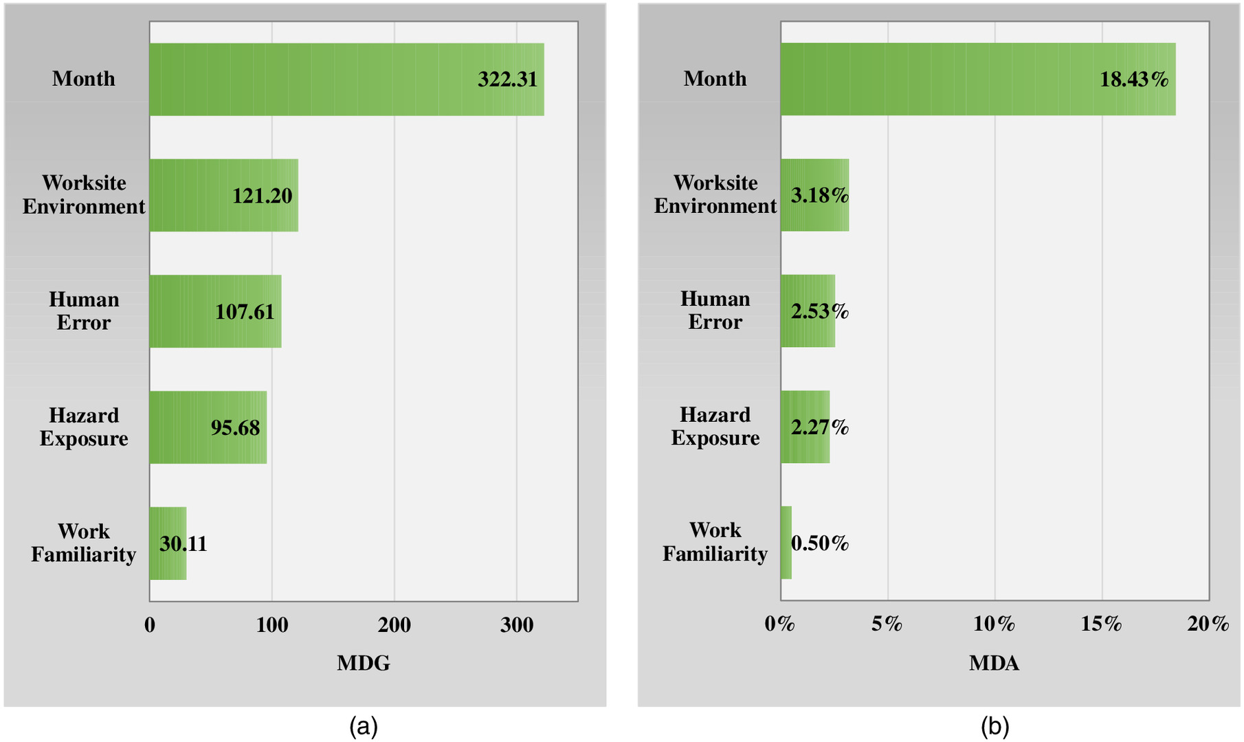
The MDA plot [Fig. 14(b)] supports the MDG plot [Fig. 14(a)], indicating that month (i.e., weather conditions) was the most important factor in construction site ISL prediction and that the CIF importance rankings in decreasing order were month, worksite environment, human error, hazard exposure, and work familiarity. Comparing the MDG results in Fig. 14(a) with the IGAE results in Fig. 8 (a method that is applied once to the entire data set), we notice two key differences: the increased relative importance of (1) month compared to other CIFs; and (2) human error, which moves up as the third-ranked CIF with an importance magnitude that becomes more comparable to worksite environment and hazard exposure. These findings suggest that, when applied repeatedly across various construction sites (i.e., as simulated by 315 bootstrap samples and trees in RF), these CIF importance patterns start to take shape. The agreement between the three variable importance algorithms [i.e., Figs. 14(a and b) and 8] on weather conditions as the key influential factor affecting ISL on sites—as well as its increasing relative magnitude when analyzed across different sites—amplifies the importance of proactive weather-specific safety planning (e.g., considering strong winds, extreme temperatures, heavy rainfall, poor weather-related visibility, etc.). For example, safety actions in inclement weather may include securing and fastening down loose objects and material, ensuring that suitable drainage channels are dug should rainfall be heavy, regulating relevant safety weather training, and planning for emergency weather evacuation. Moreover, the consistent fifth-position ranking of work familiarity across the three figures, together with the enlarged significance of human error in Fig. 14(a), suggests that, although worker/operator inexperience can be compensated by formal prejob safety trainings and certifications, site situational awareness, behavioral patterns, and mental capacity are more consistent contributors to worker negligence of controllable circumstances within their responsibilities or misjudgment of hazardous situations, ultimately leading to failure in preventing an injury/incident or mitigating its severity.
Model Performance Enhancement
To complement the RPART tree model, its ROC curve is shown in Fig. 15. For example, within the current application, the default threshold of 0.5 corresponds to a combination of FPR and TPR values of 22.58% and 85.71%, respectively, as shown in Fig. 15 and reported in Table 2. Managers may opt instead for a threshold of 0.2 and accept a reasonable increase in FPR (to 33.81%), but considerably raise TPR to 94.09%, whereas the TPR improvement due to a threshold of 0.1 does not justify the accompanying large FPR increase. A threshold of 0.2 means that terminal nodes in Fig. 13 with a fatal ISL probability of 20% or more will be designated as fatal injuries, and similarly so for the RF model. With this adjustment, managers would further improve their model’s predictive performance by reducing the more serious types of predictive errors (i.e., FNs), ultimately amplifying the impacts of their managerial actions and prevention strategies.

Site Safety Risk Level Classification
One of the developed DT- or RF-based ISL predictive models can be further integrated with another sister model that facilitates predictions of injury probability level. Together, these models can be used to quantitatively classify construction sites in accordance with their safety risk levels, thus flagging sites that are particularly associated with high risk. This site safety risk level classification can be achieved through weighting a site’s predicted ISL with the probability of an injury occurring on that site as
(10)
Although beyond the scope of the current study, which focused on ISL prediction, such a sister model can be developed from an extension to the data set used herein that considers, for example, previous construction activities/works (Gondia et al. 2022) and maps the same set of CIFs to an outcome of whether an incident/injury occurred during that work (e.g., 0 = no injury occurrence, 1 = injury occurrence). While the current demonstration data set only included cases where injuries already occurred, such an extended data set would include both injury and noninjury cases, thus supporting the development of a future predictive model that quantifies the probability of injury occurrence (i.e., in the form of a number between 0 and 1) based on a set of CIFs present on a site.
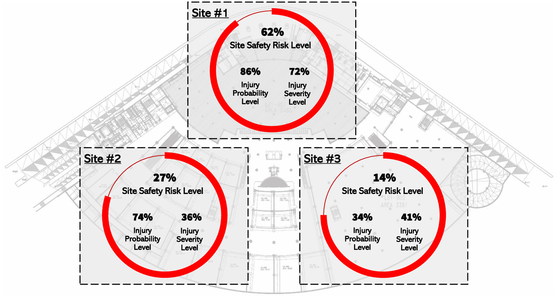
In terms of practical utilization of such two sister models, managers can qualitatively identify potential CIF categories [e.g., collected from Figs. 6(d–g)] ahead of time for a work package that is scheduled to be executed within a certain site location. This can be achieved through knowledge of the (1) time of work execution (month), (2) risks associated with the spatial working conditions relevant to the site (worksite environment), (3) nature of work and execution methods relevant to the work package (hazard exposure), and (4) assigned workers’ experience and motivation (human error and work familiarity). Using such qualitative CIF categories, managers can use the two models to quantitatively predict injury probability level and ISL outcomes, and thus classify sites as low- or high-risk zones based on Eq. (10), as illustrated for demonstration in Fig. 16. As different sets of CIFs can exist across different site locations and due to different construction works, the above-described procedure can be performed across all relevant sites, thus enabling a spatial visualization of potential site safety risk levels across the project area, as shown in Fig. 16. Empowered by such safety leading indicators and insights, managers can prioritize inspections and injury prevention strategies across high-risk sites and make proactive and better-informed decisions so that any possible risks can be mitigated before reaching the construction site.
Conclusions
Construction remains one of the most hazardous industries worldwide, but learning from past incidents is key to future injury prediction and prevention. In this regard, machine-learning-based analyses of empirical data have the potential to transform the way organizations make their safety decisions through more accurate predictions and more effective prevention. In this respect, the current study develops an interpretable machine-learning-based framework for construction injury severity prediction and subsequent risk mitigation.
Through evaluating the predictive power of different injury factors, a ranking algorithm procedure is initially utilized to pinpoint the key influential factors that safety managers can use for targeted efforts and priority actions. Subsequently, glass- and black-box models can be developed and optimized, and then used to quantitively predict injury severity levels from the combined and interdependent effects of the key identified injury factors. The model performances can then be validated through a three-tier evaluation of prediction robustness, reliability, and versatility, using multiple relevant performance evaluation measures. Receiver operating characteristics insights are also presented to aid in further adjusting model prediction thresholds to improve overall model performance according to unique safety applications and requirements. Decision support is then provided to equip managers with knowledge on when to use glass- or black-box models through a tradeoff between transparency and performance. The model-generated quantitative predictions are supported by explainable qualitative insights through leveraging the glass-box models’ transparency merits, whereas model-agnostic methods are also demonstrated to enhance black-box model interpretability, which can be useful in cases where significant performance improvements warrant selecting them over their glass-box counterparts.
A demonstration application using the OSHA injury cases data set is subsequently presented to showcase how the decision support framework can be utilized to provide safety managers with the following key insights: (1) awareness of the key influential construction injury factors at specific sites such that targeted efforts and top-priority preventive strategies can be deployed, (2) qualitative exploration of the underlying interdependence among injury factors as well as their interactive cause-and-effect relationships with injury severity (i.e., root causes of injuries), (3) guidance on identifying high-risk sites so that hazards can be eliminated proactively, thus enhancing workplace safety, (4) decision support on model selection based on a tradeoff between transparency and performance, (5) deepened understanding of machine learning model mechanisms and outputs for ultimately selecting prediction thresholds that can improve model performance by avoiding fatal injury prediction errors, and (6) improved interpretation of black-box model outcomes, which can help remove barriers to more widespread adoption of these models in construction safety research.
Notwithstanding the value of the developed machine learning models in predicting injury severity levels of construction sites based on the existence and interplay of various injury factors, the current framework also dives into the inner workings of a typical machine learning model (e.g., variable importance evaluation, cause-and-effect relationships, transparency/performance tradeoff, prediction threshold selection criteria, model-agnostic interpretability methods) in an attempt to demystify how such model predictions can be evaluated and interpreted in construction safety and engineering risk applications. Ultimately, through the ability to better understand, predict, and prevent the occurrence of construction injuries, the framework developed and described herein should empower safety managers and workplace risk practitioners with key decision-making tools that would foster safer sites and save lives.
Data Availability Statement
All data, models, or code that support the findings of this study are available from the corresponding author upon reasonable request.
Acknowledgments
The authors are grateful for the financial support of the Natural Science and Engineering Research Council of Canada (NSERC) CaNRisk-CREATE program, and the INTERFACE Institute and the INViSiONLab, both of McMaster University.
References
Abdel-Rahman, E. M., F. B. Ahmed, and R. Ismail. 2013. “Random forest regression and spectral band selection for estimating sugarcane leaf nitrogen concentration using EO-1 Hyperion hyperspectral data.” Int. J. Remote Sens. 34 (2): 712–728. https://doi.org/10.1080/01431161.2012.713142.
Abubakar, A. M., H. Karadal, S. W. Bayighomog, and E. Merdan. 2018. “Workplace injuries, safety climate and behaviors: Application of an artificial neural network.” Int. J. Occup. Saf. Ergon. 26 (4): 651–661. https://doi.org/10.1080/10803548.2018.1454635.
Aggarwal, C. C. 2015. Data mining: The textbook. New York: Springer.
Akhavian, R., and A. H. Behzadan. 2013. “Knowledge-based simulation modeling of construction fleet operations using multimodal-process data mining.” J. Constr. Eng. Manage. 139 (11): 04013021. https://doi.org/10.1061/(ASCE)CO.1943-7862.0000775.
Alkaissy, M., M. Arashpour, B. Ashuri, Y. Bai, and R. Hosseini. 2020. “Safety management in construction: 20 years of risk modeling.” Saf. Sci. 129 (Sep): 104805. https://doi.org/10.1016/j.ssci.2020.104805.
Altmann, A., L. Toloşi, O. Sander, and T. Lengauer. 2010. “Permutation importance: A corrected feature importance measure.” Bioinformatics 26 (10): 1340–1347. https://doi.org/10.1093/bioinformatics/btq134.
Arlot, S., and A. Celisse. 2010. “A survey of cross-validation procedures for model selection.” Stat. Surv. 4 (Jan): 40–79. https://doi.org/10.1214/09-SS054.
AWCBC (Association of Workers’ Compensation Boards of Canada). 2021. “National work injury, disease and fatality statistics.” Accessed August 4, 2021. https://awcbc.org/en/statistics/.
Ayhan, B. U., and O. B. Tokdemir. 2020. “Accident analysis for construction safety using latent class clustering and artificial neural networks.” J. Constr. Eng. Manage. 146 (3): 04019114. https://doi.org/10.1061/(ASCE)CO.1943-7862.0001762.
BEA (Bureau of Economic Analysis). 2021. “Employment by NAICS industry.” Accessed July 27, 2021. https://www.bea.gov/data/employment/employment-by-industry.
Behm, M. 2005. “Linking construction fatalities to the design for construction safety concept.” Saf. Sci. 43 (8): 589–611. https://doi.org/10.1016/j.ssci.2005.04.002.
Bergstra, J., and Y. Bengio. 2012. “Random search for hyper-parameter optimization.” J. Mach. Learn. Res. 13 (2): 281–305.
BLS (Bureau of Labor Statistics). 2021a. “Census of fatal occupational injuries (CFOI).” Accessed July 27, 2021. https://www.bls.gov/iif/oshcfoi1.htm.
BLS (Bureau of Labor Statistics). 2021b. “Survey of occupational injuries and illnesses data.” Accessed July 27, 2021. https://www.bls.gov/iif/soii-data.htm#dafw.
Breiman, L. 1996. “Bagging predictors.” Mach. Learn. 24 (2): 123–140. https://doi.org/10.1007/BF00058655.
Breiman, L. 2001. “Random forests.” Mach. Learn. 45 (1): 5–32. https://doi.org/10.1023/A:1010933404324.
Breiman, L., J. H. Friedman, R. A. Olshen, and C. J. Stone. 1984. Vol. 432 of Classification and regression trees, 151–166. Belmont, CA: Wadsworth International Group.
Chen, Q., and R. Jin. 2013. “Multilevel safety culture and climate survey for assessing new safety program.” J. Constr. Eng. Manage. 139 (7): 805–817. https://doi.org/10.1061/(ASCE)CO.1943-7862.0000659.
Chi, S., S.-J. Suk, Y. Kang, and S. P. Mulva. 2012. “Development of a data mining-based analysis framework for multi-attribute construction project information.” Adv. Eng. Inf. 26 (3): 574–581. https://doi.org/10.1016/j.aei.2012.03.005.
Chou, J.-S., and C. Lin. 2013. “Predicting disputes in public-private partnership projects: Classification and ensemble models.” J. Comput. Civ. Eng. 27 (1): 51–60. https://doi.org/10.1061/(ASCE)CP.1943-5487.0000197.
Choudhry, R. M., D. Fang, and H. Lingard. 2009. “Measuring safety climate of a construction company.” J. Constr. Eng. Manage. 135 (9): 890–899. https://doi.org/10.1061/(ASCE)CO.1943-7862.0000063.
Cooper, M. D., and R. A. Phillips. 2004. “Exploratory analysis of the safety climate and safety behavior relationship.” J. Saf. Res. 35 (5): 497–512. https://doi.org/10.1016/j.jsr.2004.08.004.
Dedobbeleer, N., and F. Béland. 1991. “A safety climate measure for construction sites.” J. Saf. Res. 22 (2): 97–103. https://doi.org/10.1016/0022-4375(91)90017-P.
Desai, V. S., and S. Joshi. 2010. “Application of decision tree technique to analyze construction project data.” In Proc., Int. Conf. on Information Systems, Technology and Management, 304–313. Berlin: Springer.
Fang, D., Y. Chen, and L. Wong. 2006. “Safety climate in construction industry: A case study in Hong Kong.” J. Constr. Eng. Manage. 132 (6): 573–584. https://doi.org/10.1061/(ASCE)0733-9364(2006)132:6(573).
Feng, D.-C., W.-J. Wang, S. Mangalathu, and E. Taciroglu. 2021. “Interpretable XGBoost-SHAP machine-learning model for shear strength prediction of squat RC walls.” J. Struct. Eng. 147 (11): 04021173. https://doi.org/10.1061/(ASCE)ST.1943-541X.0003115.
Feng, Y., E. A. L. Teo, F. Y. Y. Ling, and S. P. Low. 2014. “Exploring the interactive effects of safety investments, safety culture and project hazard on safety performance: An empirical analysis.” Int. J. Project Manage. 32 (6): 932–943. https://doi.org/10.1016/j.ijproman.2013.10.016.
Fiore, A., G. Quaranta, G. C. Marano, and G. Monti. 2016. “Evolutionary polynomial regression–based statistical determination of the shear capacity equation for reinforced concrete beams without stirrups.” J. Comput. Civ. Eng. 30 (1): 04014111. https://doi.org/10.1061/(ASCE)CP.1943-5487.0000450.
Friedman, J. H. 2001. “Greedy function approximation: A gradient boosting machine.” Ann. Stat. 29 (5): 1189–1232. https://doi.org/10.1214/aos/1013203451.
Gerassis, S., J. E. Martín, J. T. García, A. Saavedra, and J. Taboada. 2017. “Bayesian decision tool for the analysis of occupational accidents in the construction of embankments.” J. Constr. Eng. Manage. 143 (2): 04016093. https://doi.org/10.1061/(ASCE)CO.1943-7862.0001225.
Glendon, A. I., and D. K. Litherland. 2001. “Safety climate factors, group differences and safety behaviour in road construction.” Saf. Sci. 39 (3): 157–188. https://doi.org/10.1016/S0925-7535(01)00006-6.
Goldstein, A., A. Kapelner, J. Bleich, and E. Pitkin. 2015. “Peeking inside the black box: Visualizing statistical learning with plots of individual conditional expectation.” J. Comput. Graphical Stat. 24 (1): 44–65. https://doi.org/10.1080/10618600.2014.907095.
Gondia, A., M. Ezzeldin, and W. El-Dakhakhni. 2020. “Mechanics-guided genetic programming expression for shear-strength prediction of squat reinforced concrete walls with boundary elements.” J. Struct. Eng. 146 (11): 04020223. https://doi.org/10.1061/(ASCE)ST.1943-541X.0002734.
Gondia, A., M. Ezzeldin, and W. El-Dakhakhni. 2022. “Dynamic networks for resilience-driven management of infrastructure projects.” Auto. Constr. 136: 104149. https://doi.org/10.1016/j.autcon.2022.104149.
Gondia, A., A. Siam, W. El-Dakhakhni, and A. H. Nassar. 2019. “Machine learning algorithms for construction projects delay risk prediction.” J. Constr. Eng. Manage. 146 (1): 04019085. https://doi.org/10.1061/(ASCE)CO.1943-7862.0001736.
Gorissen, D., I. Couckuyt, P. Demeester, T. Dhaene, and K. Crombecq. 2010. “A surrogate modeling and adaptive sampling toolbox for computer based design.” J. Mach. Learn. Res. 11 (68): 2051–2055.
Hallowell, M. R., J. W. Hinze, K. C. Baud, and A. Wehle. 2013. “Proactive construction safety control: Measuring, monitoring, and responding to safety leading indicators.” J. Constr. Eng. Manage. 139 (10): 04013010. https://doi.org/10.1061/(ASCE)CO.1943-7862.0000730.
Han, T., D. Jiang, Q. Zhao, L. Wang, and K. Yin. 2018. “Comparison of random forest, artificial neural networks and support vector machine for intelligent diagnosis of rotating machinery.” Trans. Inst. Meas. Control 40 (8): 2681–2693. https://doi.org/10.1177/0142331217708242.
Hong, H., P. Tsangaratos, I. Ilia, W. Chen, and C. Xu. 2017. “Comparing the performance of a logistic regression and a random forest model in landslide susceptibility assessments. The case of Wuyaun area, China.” In Proc., Workshop on World Landslide Forum, 1043–1050. Cham, Switzerland: Springer.
Hornik, K., C. Buchta, and A. Zeileis. 2009. “Open-source machine learning: R meets Weka.” Comput. Stat. 24 (2): 225–232. https://doi.org/10.1007/s00180-008-0119-7.
Huang, L., C. Wu, B. Wang, and Q. Ouyang. 2018. “Big-data-driven safety decision-making: A conceptual framework and its influencing factors.” Saf. Sci. 109 (Nov): 46–56. https://doi.org/10.1016/j.ssci.2018.05.012.
James, G., D. Witten, T. Hastie, and R. Tibshirani. 2013. Vol. 112 of An introduction to statistical learning, 3–7. New York: Springer.
Jin, R., P. X. Zou, P. Piroozfar, H. Wood, Y. Yang, L. Yan, and Y. Han. 2019. “A science mapping approach based review of construction safety research.” Saf. Sci. 113 (Mar): 285–297. https://doi.org/10.1016/j.ssci.2018.12.006.
Kakhki, F. D., S. A. Freeman, and G. A. Mosher. 2019. “Evaluating machine learning performance in predicting injury severity in agribusiness industries.” Saf. Sci. 117 (Aug): 257–262. https://doi.org/10.1016/j.ssci.2019.04.026.
Kang, K., and H. Ryu. 2019. “Predicting types of occupational accidents at construction sites in Korea using random forest model.” Saf. Sci. 120 (Dec): 226–236. https://doi.org/10.1016/j.ssci.2019.06.034.
Kohavi, R. 1995. “A study of cross-validation and bootstrap for accuracy estimation and model selection.” In Vol. 14 of Proc., IJCAI’95: Proc. of the 14th Int. Joint Conf. On Artificial Intelligence, 1137–1145. Menlo Park, CA: American Association for Artificial Intelligence.
Kuhn, M., and K. Johnson. 2013. “Measuring performance in classification models.” In Applied predictive modeling, 247–273. New York: Springer.
Li, Z., P. Liu, W. Wang, and C. Xu. 2012. “Using support vector machine models for crash injury severity analysis.” Accid. Anal. Prev. 45 (Mar): 478–486. https://doi.org/10.1016/j.aap.2011.08.016.
Liu, X., Y. Song, W. Yi, X. Wang, and J. Zhu. 2018. “Comparing the random forest with the generalized additive model to evaluate the impacts of outdoor ambient environmental factors on scaffolding construction productivity.” J. Constr. Eng. Manage. 144 (6): 04018037. https://doi.org/10.1061/(ASCE)CO.1943-7862.0001495.
Lundberg, S. M., G. Erion, H. Chen, A. DeGrave, J. M. Prutkin, B. Nair, R. Katz, J. Himmelfarb, N. Bansal, and S.-I. Lee. 2020. “From local explanations to global understanding with explainable AI for trees.” Nat. Mach. Intell. 2 (1): 56–67. https://doi.org/10.1038/s42256-019-0138-9.
Lundberg, S. M., and S.-I. Lee. 2017. “A unified approach to interpreting model predictions.” In Proc., 31st Int. Conf. on Neural Information Processing Systems, 4768–4777. Vancouver, BC, Canada: NeurIPS.
Makki, A. A., and I. Mosly. 2021. “Predicting the safety climate in construction sites of Saudi Arabia: A bootstrapped multiple ordinal logistic regression modeling approach.” Appl. Sci. 11 (4): 1474. https://doi.org/10.3390/app11041474.
Marin, L. S., H. Lipscomb, M. Cifuentes, and L. Punnett. 2019. “Perceptions of safety climate across construction personnel: Associations with injury rates.” Saf. Sci. 118 (Oct): 487–496. https://doi.org/10.1016/j.ssci.2019.05.056.
Mattila, M., M. Hyttinen, and E. Rantanen. 1994. “Effective supervisory behaviour and safety at the building site.” Int. J. Ind. Ergon. 13 (2): 85–93. https://doi.org/10.1016/0169-8141(94)90075-2.
McDonald, N., S. Corrigan, C. Daly, and S. Cromie. 2000. “Safety management systems and safety culture in aircraft maintenance organisations.” Saf. Sci. 34 (1–3): 151–176. https://doi.org/10.1016/S0925-7535(00)00011-4.
Mearns, K., S. M. Whitaker, and R. Flin. 2003. “Safety climate, safety management practice and safety performance in offshore environments.” Saf. Sci. 41 (8): 641–680. https://doi.org/10.1016/S0925-7535(02)00011-5.
Mohamed, S. 2002. “Safety climate in construction site environments.” J. Constr. Eng. Manage. 128 (5): 375–384. https://doi.org/10.1061/(ASCE)0733-9364(2002)128:5(375).
Mohammadi, A., M. Tavakolan, and Y. Khosravi. 2018. “Factors influencing safety performance on construction projects: A review.” Saf. Sci. 109 (Nov): 382–397. https://doi.org/10.1016/j.ssci.2018.06.017.
Molnar, C. 2020. “Interpretable machine learning: A guide for making black box models explainable.” Accessed January 15, 2021. https://christophm.github.io/interpretable-ml-book.
Naser, M. Z. 2021. “An engineer’s guide to eXplainable artificial intelligence and interpretable machine learning: Navigating causality, forced goodness, and the false perception of inference.” Autom. Constr. 129 (Sep): 103821. https://doi.org/10.1016/j.autcon.2021.103821.
Nyshadham, C., M. Rupp, B. Bekker, A. V. Shapeev, T. Mueller, C. W. Rosenbrock, G. Csányi, D. W. Wingate, and G. L. Hart. 2019. “Machine-learned multi-system surrogate models for materials prediction.” NPJ Comput. Mater. 5 (1): 1–6. https://doi.org/10.1038/s41524-019-0189-9.
OSHA (Occupational Safety and Health Administration). 2019. “Injuries, illnesses, and fatalities.” Accessed February 17, 2019. https://www.bls.gov/iif/oshoiics.htm.
OSHA (Occupational Safety and Health Administration). 2021. “Recommended practices for safety and health programs.” Accessed April 6, 2021. https://www.osha.gov/safety-management.
Patel, D. A., and K. N. Jha. 2015. “Neural network approach for safety climate prediction.” J. Manage. Eng. 31 (6): 05014027. https://doi.org/10.1061/(ASCE)ME.1943-5479.0000348.
Pereira, E., S. Ahn, S. Han, and S. Abourizk. 2018. “Identification and association of high-priority safety management system factors and accident precursors for proactive safety assessment and control.” J. Manage. Eng. 34 (1): 04017041. https://doi.org/10.1061/(ASCE)ME.1943-5479.0000562.
Pereira, E., S. Ahn, S. Han, and S. Abourizk. 2020. “Finding causal paths between safety management system factors and accident precursors.” J. Manage. Eng. 36 (2): 04019049. https://doi.org/10.1061/(ASCE)ME.1943-5479.0000738.
Poh, C. Q. X., C. U. Ubeynarayana, and Y. M. Goh. 2018. “Safety leading indicators for construction sites: A machine learning approach.” Autom. Constr. 93 (Sep): 375–386. https://doi.org/10.1016/j.autcon.2018.03.022.
Ripley, B. 2018. “Classification and regression trees: R package version 1.0-39.” Accessed August 10, 2018. https://CRAN.R-project.org/package=tree.
Rodriguez-Galiano, V., M. P. Mendes, M. J. Garcia-Soldado, M. Chica-Olmo, and L. Ribeiro. 2014. “Predictive modeling of groundwater nitrate pollution using random forest and multisource variables related to intrinsic and specific vulnerability: A case study in an agricultural setting (southern Spain).” Sci. Total Environ. 476 (Apr): 189–206. https://doi.org/10.1016/j.scitotenv.2014.01.001.
Rodriguez-Galiano, V. F., B. Ghimire, J. Rogan, M. Chica-Olmo, and J. P. Rigol-Sanchez. 2012. “An assessment of the effectiveness of a random forest classifier for land-cover classification.” ISPRS J. Photogramm. Remote Sens. 67 (Jan): 93–104. https://doi.org/10.1016/j.isprsjprs.2011.11.002.
Sakhakarmi, S., J. Park, and C. Cho. 2019. “Enhanced machine learning classification accuracy for scaffolding safety using increased features.” J. Constr. Eng. Manage. 145 (2): 04018133. https://doi.org/10.1061/(ASCE)CO.1943-7862.0001601.
Seong, H., H. Son, and C. Kim. 2018. “A comparative study of machine learning classification for color-based safety vest detection on construction-site images.” KSCE J. Civ. Eng. 22 (11): 4254–4262. https://doi.org/10.1007/s12205-017-1730-3.
Shannon, C. E. 1948. “A mathematical theory of communication, Part I, Part II.” Bell Syst. Tech. J. 27 (3): 623–656. https://doi.org/10.1002/j.1538-7305.1948.tb00917.x.
Siam, A., M. Ezzeldin, and W. El-Dakhakhni. 2019. “Machine learning algorithms for structural performance classifications and predictions: Application to reinforced masonry shear walls.” Structures 22 (Dec): 252–265. https://doi.org/10.1016/j.istruc.2019.06.017.
Son, H., C. Kim, N. Hwang, C. Kim, and Y. Kang. 2014. “Classification of major construction materials in construction environments using ensemble classifiers.” Adv. Eng. Inf. 28 (1): 1–10. https://doi.org/10.1016/j.aei.2013.10.001.
Statistics Canada. 2021. “Labour force characteristics by industry annual (×1,000).” Accessed August 4, 2021. https://www150.statcan.gc.ca/t1/tbl1/en/tv.action?pid=1410002301.
Štrumbelj, E., and I. Kononenko. 2014. “Explaining prediction models and individual predictions with feature contributions.” Knowl. Inf. Syst. 41 (3): 647–665. https://doi.org/10.1007/s10115-013-0679-x.
Sutton, C. D. 2005. “Classification and regression trees, bagging, and boosting.” In Vol. 24 of Handbook of statistics, 303–329.
Therneau, T., and B. Atkinson. 2018. “Recursive partitioning and regression trees: R package version 4.1-13.” Accessed August 10, 2018. https://CRAN.R-project.org/package=rpart.
Tixier, A. J.-P., M. R. Hallowell, B. Rajagopalan, and D. Bowman. 2016. “Application of machine learning to construction injury prediction.” Autom. Constr. 69 (Sep): 102–114. https://doi.org/10.1016/j.autcon.2016.05.016.
Wang, W., X. Jiang, S. Xia, and Q. Cao. 2010. “Incident tree model and incident tree analysis method for quantified risk assessment: An in-depth accident study in traffic operation.” Saf. Sci. 48 (10): 1248–1262. https://doi.org/10.1016/j.ssci.2010.04.002.
Zhang, Y., A. Javanmardi, Y. Liu, S. Yang, X. Yu, S. M. Hsiang, Z. Jiang, and M. Liu. 2020. “How does experience with delay shape managers’ making-do decision: Random forest approach.” J. Manage. Eng. 36 (4): 04020030. https://doi.org/10.1061/(ASCE)ME.1943-5479.0000776.
Zhou, J., X. Li, and H. S. Mitri. 2016. “Classification of rockburst in underground projects: Comparison of ten supervised learning methods.” J. Comput. Civ. Eng. 30 (5): 04016003. https://doi.org/10.1061/(ASCE)CP.1943-5487.0000553.
Zhou, Y., S. Li, C. Zhou, and H. Luo. 2019. “Intelligent approach based on random forest for safety risk prediction of deep foundation pit in subway stations.” J. Comput. Civ. Eng. 33 (1): 05018004. https://doi.org/10.1061/(ASCE)CP.1943-5487.0000796.
Zhou, Y., W. Su, L. Ding, H. Luo, and P. E. Love. 2017. “Predicting safety risks in deep foundation pits in subway infrastructure projects: Support vector machine approach.” J. Comput. Civ. Eng. 31 (5): 04017052. https://doi.org/10.1061/(ASCE)CP.1943-5487.0000700.
Zohar, D. 1980. “Safety climate in industrial organizations: Theoretical and applied implications.” J. Appl. Psychol. 65 (1): 96. https://doi.org/10.1037/0021-9010.65.1.96.
Zohar, D. 2002. “The effects of leadership dimensions, safety climate, and assigned priorities on minor injuries in work groups.” J. Organizational Behav. 23 (1): 75–92. https://doi.org/10.1002/job.130.
Information & Authors
Information
Published In

ASCE-ASME Journal of Risk and Uncertainty in Engineering Systems, Part A: Civil Engineering
Volume 8 • Issue 3 • September 2022
Copyright
This work is made available under the terms of the Creative Commons Attribution 4.0 International license, https://creativecommons.org/licenses/by/4.0/.
History
Received: Sep 9, 2021
Accepted: Feb 10, 2022
Published online: May 6, 2022
Published in print: Sep 1, 2022
Discussion open until: Oct 6, 2022
ASCE Technical Topics:
- Artificial intelligence and machine learning
- Business management
- Computer programming
- Computing in civil engineering
- Construction engineering
- Construction equipment
- Construction management
- Construction sites
- Disaster risk management
- Engineering fundamentals
- Equipment and machinery
- Managers
- Mitigation and remediation
- Models (by type)
- Occupational safety
- Optimization models
- Personnel (type)
- Personnel management
- Practice and Profession
- Public administration
- Public health and safety
- Risk management
- Safety
Authors
Metrics & Citations
Metrics
Citations
Download citation
If you have the appropriate software installed, you can download article citation data to the citation manager of your choice. Simply select your manager software from the list below and click Download.
Cited by
- Qianmai Luo, Chengshuang Sun, Ying Li, Zhenqiang Qi, Guozong Zhang, Applications of digital twin technology in construction safety risk management: a literature review, Engineering, Construction and Architectural Management, 10.1108/ECAM-11-2023-1095, (2024).
- Xi Pan, Tingsheng Zhao, Xiaowei Li, Zibo Zuo, Gang Zong, Longlong Zhang, Automatic Identification of the Working State of High-Rise Building Machine Based on Machine Learning, Applied Sciences, 10.3390/app132011411, 13, 20, (11411), (2023).
- Kerim Koc, Role of National Conditions in Occupational Fatal Accidents in the Construction Industry Using Interpretable Machine Learning Approach, Journal of Management in Engineering, 10.1061/JMENEA.MEENG-5516, 39, 6, (2023).
- Kerim Koc, Ömer Ekmekcioğlu, Asli Pelin Gurgun, Developing a National Data-Driven Construction Safety Management Framework with Interpretable Fatal Accident Prediction, Journal of Construction Engineering and Management, 10.1061/JCEMD4.COENG-12848, 149, 4, (2023).
- Ansa Varghese, Bino I. Koshy, Risk perception on building construction safety, Materials Today: Proceedings, 10.1016/j.matpr.2023.04.070, (2023).
- Yaren Aydin, Gebrail Bekdaş, Ümit Işıkdağ, Sinan Melih Nigdeli, The State of Art in Machine Learning Applications in Civil Engineering, Hybrid Metaheuristics in Structural Engineering, 10.1007/978-3-031-34728-3_9, (147-177), (2023).
- Lan Wu, Qi Shen, Gen Li, Identifying Risk Factors for Autos and Trucks on Highway-Railroad Grade Crossings Based on Mixed Logit Model, International Journal of Environmental Research and Public Health, 10.3390/ijerph192215075, 19, 22, (15075), (2022).
- Zhi-Jun Chen, Tsung-Shun Hsieh, Seyed Mehdi Mousavi Davoudi, Analysis of Factors Affecting the Success of Sustainable Development Projects with the Help of Machine Learning Tools, Discrete Dynamics in Nature and Society, 10.1155/2022/1956879, 2022, (1-9), (2022).