Earthquake Risk of Gas Pipelines in the Conterminous United States and Its Sources of Uncertainty

We utilized the US Geological Survey (USGS) 2018 National Seismic Hazard Model (NSHM) (Petersen et al. 2019) to quantify the aleatory variability of seismic hazard for strong ground shaking at the national scale. The 2018 NSHM does not provide seismic hazard for PGV (Powers et al., forthcoming), so we estimate it from 5%-damped spectral acceleration at a vibration period of 1 s using the Hazus methodology (FEMA 2012; Mousavi et al. 2014). Previous research has shown that hazard curves based only on reference soil conditions (i.e., $V_{S30}=760\mathrm{m}/\mathrm{s}$) tend to underestimate the annualized earthquake losses (Jaiswal et al. 2015). To account for local soils, we first estimate the site-specific value of $V_{S30}$ using the USGS global server (Wald and Allen 2007) at the midpoint of each pipeline segment. Then, we applied linear interpolation of $V_{S30}$ and logarithmic interpolation of exceedance frequencies to the $V_{S30}$-specific hazard curves from the 2018 NSHM (Shumway et al. 2021). The resulting hazard curves serve as best estimates of ${\hat{H}}_s(v)$ in Eq. (6).

Fig. 1 presents the estimated PGV hazard curves at four cities across the CONUS using each city’s estimate of $V_{S30}$, which are shown in the legend. While the highest hazard in this figure corresponds to Los Angeles, the lowest hazard corresponds to Chicago. However, being situated in the central or eastern US does not necessarily imply low seismic hazard because the hazard for Memphis, which is near the NMSZ, exceeds that for Portland, at exceedance frequencies that are lower than $\sim 4\times {10}^{-3}$. Therefore, the earthquake threat for gas transmission pipelines is a national concern.

When estimating AAL using Eq. (6), the estimated PGV hazard curve for a given pipeline segment, ${\hat{H}}_s(v)$, contains epistemic uncertainty because of limited data and knowledge in characterizing the seismic sources and defining the ground motion model (Kiureghian and Ditlevsen 2009; McGuire 2004). Furthermore, this epistemic uncertainty increases for increasing levels of seismic hazard. This feature implies larger uncertainty for low-probability-high-consequence events (e.g., large RRs associated with rare PGV exceedance) than for high-probability-low-consequence events (e.g., small RRs associated with frequent PGV exceedance).

The 2018 NSHM does not provide estimates of epistemic uncertainty in seismic hazard, so we estimate it by first assuming that the annual exceedance frequency at a given PGV level is lognormally distributed (Bradley 2009; Lee et al. 2018) and then estimating the logarithmic standard deviation as a function of annual exceedance frequency. While the annual exceedance frequency may not strictly follow a lognormal distribution (e.g., Lacour and Abrahamson 2019), the lognormal assumption facilitates capturing the center, body, and range of technically defensible interpretations of data (Atkinson et al. 2014). The probabilistic seismic hazard analysis conducted for Yucca Mountain, NV, in Stepp et al. (2001) was one of the most comprehensive analyses because it rigorously captured epistemic uncertainty in the seismic source characterization through six teams of experts on seismic sources and epistemic uncertainty in ground motion model through seven experts on ground motions. Therein, their Fig. 10(b) documents several “fractiles” for the annual probability of exceeding spectral acceleration at 1 s. Assuming that probabilities are approximately equal to frequencies and data for 1-s spectral acceleration are applicable to PGV, their Fig. 10(b) essentially portrays a realistic estimate of epistemic uncertainties in hazard. Based on that figure, we created a model to approximately estimate the logarithmic standard deviation of annual exceedance frequency, denoted by ${\sigma }_{\ln H}$, as a function of annual exceedance frequency, $H$. Specifically, we assume a constant epistemic uncertainty of ${\sigma }_{\ln H}=0.67$ for annual frequencies of 0.01 or higher, whereas for lower annual frequencies, the epistemic uncertainty increases linearly to a value of ${\sigma }_{\ln H}=1.6$ at an annual frequency of $1.7\times {10}^{-6}$.

We applied this approximate model for ${\sigma }_{\ln H}$ to all estimated PGV hazard curves in the CONUS to study epistemic uncertainty in seismic hazard and its impact on the resulting risk. For a given site, we used the approximate model for ${\sigma }_{\ln H}$ to determine the median hazard curve; this assumes that the previously estimated PGV hazard curve corresponds to the mean (Abrahamson and Bommer 2005; McGuire et al. 2005) and that the annual exceedance frequency at a given PGV level is lognormally distributed. Next, we determine various percentiles (e.g., 85, 97.5) of hazard curves by multiplying the median hazard curve with $\exp [{\mathrm{\Phi }}^{-1}(p){\sigma }_{\ln H}]$ where ${\mathrm{\Phi }}^{-1}(p)$ denotes the inverse of the standard normal cumulative distribution function at the specified $p$th percentile. Because the mean hazard curve from the 2018 NSHM varies spatially with different locations, the percentile hazard curves also vary spatially with different sites.

As examples, Fig. 1 presents 15 and 85 percentile curves for each of the four cities. The 85-percentile curve for Memphis, TN, exceeds the 15-percentile curve for Los Angeles, CA, at annual frequencies lower than ${10}^{-3}$, highlighting the importance of quantifying epistemic uncertainty in seismic hazard when quantifying risk. The figure also shows that the approximate model for ${\sigma }_{\ln H}$ captures increasing epistemic uncertainty for increasing levels of hazard. However, our estimate of epistemic uncertainty in seismic hazard, ${\sigma }_{\ln H}$, is based on a comprehensive analysis of one location in NV, which may not be accurate for other sites. While we have also considered other choices for estimating this epistemic uncertainty [e.g., trying an approximate model based on data from Bradley (2009)], improved estimates will better inform the subsequent sensitivity analyses.

The locations of gas pipelines are sensitive information even though they are necessary inputs for seismic risk assessments (Applied Technology Council 2016). Fortunately, PHMSA annually collects this information from operators in a standardized format (Pipeline and Hazardous Materials Safety Administration 2017). Access to the 2018 National Pipeline Mapping System (NPMS) dataset of gas transmission pipelines in the CONUS was obtained through a confidential agreement with PHMSA. This dataset provides input pipeline attributes $\mathit{\theta }$ such as geographic location, total mileage, managing operator, classification of interstate versus intrastate, or commodity. However, many other pipeline attributes that are needed to develop an engineering exposure model and estimate potential seismic damage are unavailable (e.g., burial depth and decade of installation are unknown for all segments). Pipe diameter is available for 58.4% of the total mileage because operators were not required to provide this information.

We supplemented information from the NPMS dataset by compiling and analyzing annual reports that are submitted by pipeline operators to PHMSA (Pipeline and Hazardous Materials Safety Administration 2020b). These reports provide distributions of total mileage by pipe diameter, pipe material, and decade of installation for each operator’s assets. For 2018, we found that 99.5% of the total pipeline mileage is made of steel and that almost all have some form of protection against corrosion. Moreover, the next dominant category of pipe material is plastic, and none of the transmission lines are made of cast iron, which differs from gas distribution lines. We also found that 3.79% of the total mileage was essentially installed before 1940, which roughly distinguishes pipeline response from brittle versus ductile behavior (FEMA 2012; O’Rourke and Palmer 1996).

One of the most important pipeline attributes that is missing in the NPMS dataset is the classification of a pipeline segment as an HCA (49 C.F.R. § 192.903). Due to the importance of HCAs, we discretized all pipeline segments in the NPMS dataset that are longer than 1.6 km (1 mi.) into segments whose length $l_s$ is 1.6 km (1 mi.) long or shorter (ASME 2018). We used this discretization and data on nearby buildings to approximately classify each segment as either HCA or non-HCA, but this effort is not discussed further due to space limitations. Based on PHMSA annual reports for 2018, approximately 6.89% of all mileage for onshore gas transmission pipelines in the CONUS corresponds to HCAs. Moreover, the top five states with the largest share of the total HCA mileage are CA (15.0%), TX (13.4%), IL (5.51%), PA (5.42%), and FL (4.12%). For context, the corresponding share of the total mileage in these states are CA (4.13%), TX (15.4%), IL (3.09%), PA (3.48%), and FL (1.83%). These statistics show that in addition to operators in CA, operators in other states such as TX or PA are also required to consider seismicity in their Integrity Management Programs, highlighting the need to better understand earthquake risk of gas pipelines at the national scale.

In addition to epistemic uncertainty in hazard curves, the epistemic uncertainty in pipeline attributes ${\hat{\mathit{\theta }}}_s$ also contributes to the overall uncertainty in the risk estimates [Eq. (5)]. For example, a different decade of installation leads to a different vulnerability, and hence risk. This source of uncertainty is characterized as epistemic (Kiureghian and Ditlevsen 2009) because it can be reduced by acquiring more information from the operator.

To capture this source of uncertainty, we propose a logic tree framework where each node in the logic tree of a given pipeline segment corresponds to a unique pipeline attribute [Eq. (6)]. Specifically, Table 1 presents the default nodes and branches chosen based on data available from PHMSA annual reports (Pipeline and Hazardous Materials Safety Administration 2020b). For a given node, all branches are mutually exclusive and collectively exhaustive. Therefore, the final ($9\times 9\times 28=\mathrm{2,268}$) branches are also mutually exclusive and collectively exhaustive. These branches are denoted as “default” because a vulnerability model may indicate that only a subset may be relevant in terms of estimating RRs.

While all pipeline segments share a common set of final branches, the segments’ known attributes from NPMS (i.e., operator, state, interstate classification, and commodity) determine the appropriate branch probabilities ${\hat{p}}_{s,b}$. The PHMSA 2018 annual reports provide distributions of pipeline mileage by pipeline attribute, and these distributions vary depending on the operator, state, interstate classification, and commodity. For example, the thin orange lines in Fig. 2 show the distribution of mileage by diameter for natural gas intrastate pipelines from an operator with the most HCA mileage in CA. This distribution reveals that slightly more than 60% of the mileage corresponds to diameters of 610 mm (24 in.) or less. In contrast, interstate pipelines in CA (thick orange lines in Fig. 2) are generally larger in diameter with a most likely value of approximately 762 mm (30 in.). Several more distributions for other combinations are also shown in the figure. We used a segment’s known attributes from the NPMS to determine the appropriate branch probabilities for the given node, which approximately captures correlations between segments (e.g., two adjacent intrastate segments in CA that are managed by the same operator would share the same distribution of diameter). Repeating this process for the other nodes (i.e., pipeline attributes) and assuming each node is conditionally independent of the other nodes leads to the final set of branch probabilities ${\hat{p}}_{s,b}$ for a given segment.

Considering all possibilities using the proposed logic tree framework in Eq. (6) provides a flexible way to update the exposure model given new information. For example, if the diameter of a segment is known with certainty, a value of unity can be assigned to the corresponding diameter branch in the logic tree, while zeros can be assigned to the remaining diameter branches. In this sense, the uncertainty in exposure model is epistemic in nature. Most importantly, expressing AAL via Eq. (6) instead of Eq. (5) enables conducting sensitivity analyses with realistic values of the exposure model (i.e., varying attributes only for segments in which nonzero probability exists for more than one branch).

Due to mutual exclusivity and collective exhaustivity, the default logic tree (Table 1) can be readily modified to improve computational efficiency when applying different vulnerability models for estimating RRs. For example, Fig. 3 illustrates an example logic tree for a given pipeline segment where the hypothetical vulnerability model captures the effects from decade of installation, pipe material, and pipe diameter using only four different time intervals, two different materials, and four different ranges of diameter (i.e., a total of 32 branches). Instead of applying the vulnerability model to all 2,268 branches, one can equivalently first combine and reweigh the relevant branches before applying the vulnerability model.

In earthquake engineering of gas pipelines, there are essentially two categories of models for estimating potential seismic damage: empirical RR models (e.g., American Lifelines Alliance 2001; Eidinger 2020; FEMA 2012; O’Rourke 2014) and numerical fragility models (e.g., Ashrafi et al. 2019; Jahangiri and Shakib 2018; Lee et al. 2016; Tsinidis et al. 2020b; Yoon et al. 2019). Empirical RR models are typically developed from observed damage to pipelines in past earthquakes and yield the average number of repairs per length of pipe, $RR(v,\mathit{\theta })$. Given strong ground shaking, common practice is to assume that 80% of repairs corresponds to leaks, whereas 20% of repairs corresponds to breaks (FEMA 2012; Pineda-Porras and Najafi 2010; De Risi et al. 2018) because repair records after earthquakes do not always provide enough information to distinguish between different damage states (O’Rourke 2014). Therefore, the RR functions in Eq. (6) can be expressed as ${\widetilde{RR}}_{\mathrm{leak}}(v,{\mathit{\theta }}_{s,b})=\widetilde{RR}(v,{\mathit{\theta }}_{s,b})·0.8$ and ${\widetilde{RR}}_{\mathrm{break}}(v,{\mathit{\theta }}_{s,b})=\widetilde{RR}(v,{\mathit{\theta }}_{s,b})·0.2$. In contrast, numerical fragility models are typically developed from finite-element simulations of gas pipelines subjected to a range of conditions and yield probabilities of damage state exceedance, $\mathrm{Pr}(DS\ge ds|v,\mathit{\theta })$. While exceedance probabilities can be readily used to obtain the occurrence probability for a given damage state, $\mathrm{Pr}(DS=ds|v,\mathit{\theta })$, these probabilities do not directly provide the expected number of damage state occurrences along a pipeline. One way of potentially applying fragility models for regional seismic risk assessments is to model the occurrence of damage along the pipeline as a binomial process using segments of length equal to that used in the development of the fragility model. For example, 1-km-long pipelines were studied in Jahangiri and Shakib (2018), and hence, the RR functions in Eq. (6) might alternatively be expressed as ${\widetilde{RR}}_{\mathrm{leak}}(v,{\mathit{\theta }}_{s,b})=\widetilde{\mathrm{Pr}}(DS=\mathrm{leak}|v,{\mathit{\theta }}_{s,b})/1\mathrm{km}$ and ${\widetilde{RR}}_{\mathrm{break}}(v,{\mathit{\theta }}_{s,b})=\widetilde{\mathrm{Pr}}(DS=\mathrm{break}|v,{\mathit{\theta }}_{s,b})/1\mathrm{km}$; however, this approach implies an upper limit of one repair per kilometer, which might be reasonable for some but not all values of PGV (e.g., Table 3 in O’Rourke and Palmer 1996).

There are both advantages and disadvantages to empirical RR models. For example, they are commonly used in regional seismic risk assessments of pipelines, including gas pipelines (Ameri and van de Lindt 2019; Esposito et al. 2013, 2015; Gehl et al. 2014; Jahangiri and Shakib 2018; Mousavi et al. 2014; De Risi et al. 2018; Shabarchin and Tesfamariam 2017). Furthermore, they are developed empirically from observed damage in past earthquakes. However, such data are almost exclusively from water pipelines, and hence, the resulting models may not be directly applicable to gas pipelines (Honegger and Wijewickreme 2013; Karamanos et al. 2017; Tsinidis et al. 2019). Additionally, empirical RR models do not directly distinguish between different degrees of seismic damage (e.g., leak versus break) and cannot be used for strain- or stress-based design of gas pipelines.

Similarly, there are both advantages and disadvantages to numerical fragility models. For example, they are directly applicable to gas pipelines (e.g., representative joint types, grades of steel, wall thicknesses, operating pressures) and distinguish directly between different degrees of seismic damage. Furthermore, they typically capture a variety of input pipeline attributes that may impact seismic performance. However, numerical fragility models may not be directly applicable to regional seismic risk assessments because the key output is exceedance probability instead of RR. Strictly speaking, while numerical fragility models are directly applicable to gas pipelines, each model is applicable only to the specific conditions for which the model was developed [e.g., in the case of Tsinidis et al. (2020b), buried gas transmission pipelines that cross locations of vertical geotechnical discontinuities].

Given this context, we focus on two empirical RR models that have been accepted by the profession for regional seismic risk assessment of gas pipelines. The first model is the one that has been adopted into the Hazus methodology (Esposito et al. 2015; FEMA 2012; Mousavi et al. 2014; O’Rourke and Ayala 1993). In this model, the estimated RR is a function of pipeline ductility in addition to PGV. A “ductile” pipeline is defined in Hazus as one that is made of ductile material (e.g., steel with arc-welded joints), whereas other materials, including steel with gas-welded joints, are classified as “brittle” (page 8-17 in FEMA 2012). The second model is the “X grade” version of the model by the American Lifelines Alliance (ALA) 2001 [page 42 in American Lifelines Alliance (2001)]. In this model, the RR function is based on the cast iron damage algorithm for unknown soil conditions but scaled by 0.01 to reflect the general quality controls and design procedures that are commonly used for gas pipelines. This X grade version is a function of PGV only and differs from the “welded steel” versions in Tables 4 and 5 of the same reference, which are intended for construction characteristics that are typical of water pipelines (American Lifelines Alliance 2001).

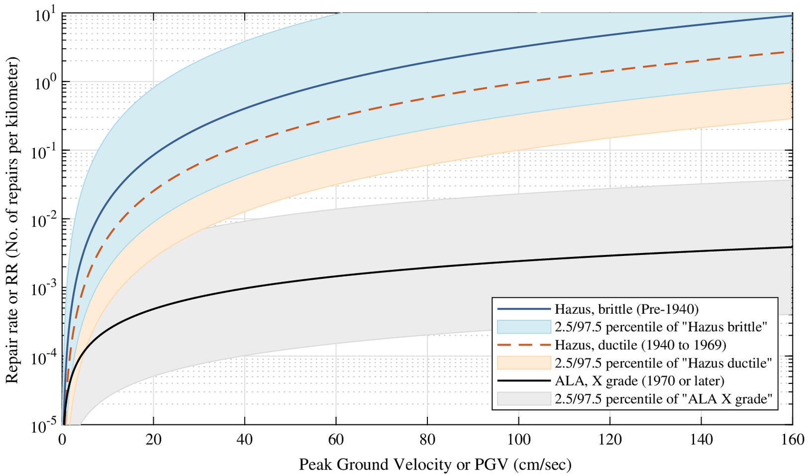
The preceding two empirical RR models are illustrated in Fig. 4. While the ductile curve from Hazus is lower than the brittle curve, it greatly exceeds the X grade curve from ALA. This level of difference highlights relatively large uncertainty in the estimated RR, even when both the level of PGV and the type of joint (e.g., not gas-welded) are known.

Empirical evidence for gas transmission pipelines suggests that both vulnerability models may be plausible. On the one hand, the Hazus model seems plausible because relatively high RRs have indeed been observed for gas transmission pipelines in past earthquakes. For example, Table 3 in O’Rourke and Palmer (1996) shows that in areas with no reported permanent ground deformation during the 1994 Northridge earthquake, a RR of 0.27 repairs per kilometer was observed for Line No. 1001, which was installed in 1925, joined by oxy-acetylene welds, and damaged by transient ground deformations (Honegger 2000). Similarly, the same table shows that in the 1971 San Fernando earthquake, a RR of 1.03 repairs per kilometer was observed for Line No. 102.90, which was installed in 1920–1921 and joined by oxy-acetylene welds. Using the USGS ShakeMaps (Wald et al. 2005) for these two earthquakes as well as the approximate locations of these repairs depicted in Figs. 3 and 6 from O’Rourke and Palmer (1996), a PGV range of 20 to $50\mathrm{cm}/\mathrm{s}$ was estimated for the RR of 0.27, and a PGV range of 70 to $220\mathrm{cm}/\mathrm{s}$ was estimated for the RR of 1.03, lending plausibility to both curves from Hazus.

On the other hand, the ALA X grade model also seems plausible because gas transmission pipelines have rarely been damaged by strong ground shaking in past earthquakes. For example, Table 3 in O’Rourke and Palmer (1996) shows one instance of no damage in the 1933 Long Beach earthquake, five instances of no damage in the 1952 and 1954 Kern County earthquakes, one instance of no damage in the 1971 San Fernando earthquake, and three instances of no damage in the 1994 Northridge earthquake. Furthermore, unlike the gas distribution system (Honegger 1998), the gas transmission system in San Francisco was virtually undamaged during the 1989 Loma Prieta earthquake (National Research Council 1994, p. 140). Similarly, no leaks were found for gas transmission pipelines after the 2019 Ridgecrest earthquake sequence (Jacobson 2019). These data lend plausibility to the X grade curve from ALA.

As noted on page 494 of O’Rourke and Palmer (1996), in which the authors reviewed the earthquake performance of gas transmission pipelines over a period of 61 years, the higher incidence of oxy-acetylene weld damage is associated with the construction quality (e.g., poor root penetration, lack of good fusion between pipe and weld), rather than the type of weld (e.g., oxy-acetylene weld versus electric arc weld), although the two aspects are related (e.g., administering welds with an oxy-acetylene torch may cause poor construction quality). Consequently, we reviewed the literature on construction practices, revealing several key milestones that may impact the construction quality of gas transmission pipelines. For example, shielded-metal-arc welding started becoming the standard approach for joining pipes in the field around the 1930s, replacing acetylene girth welds (Kiefner and Rosenfeld 2012, p. 29). Later, the time period of 1949 to 1962 was characterized by huge growth in pipe manufacturing, with new processes being developed and implemented. In 1955, the ASME standard B31 was revised, and for the first time, this revised ASME standard required recordkeeping of welding procedure qualification tests (Rosenfeld and Gailing 2013, p. 13) and hydrostatic pressure testing of pipelines before their operation; however, no duration of the pressure testing was specified at that time (Jacobs Consultancy Inc. and Gas Transmission Systems Inc 2013). In 1961, the CA Public Utilities Commission established state regulations (General Order 112) that required hydrostatic pressure testing of newly constructed pipelines for at least 1 h (Rosenfeld and Gailing 2013). In 1970, the federal safety regulations for gas transmission pipelines were issued, setting minimum requirements for designing, constructing, operating, and maintaining gas transmission pipelines across the nation. These minimum requirements include additional recordkeeping beyond that for welding and hydrostatic pressure testing of newly constructed pipelines for at least 8 h. In summary, pipelines constructed since 1970 represent state of the art in metallurgy of steel, pipe mill practices, and construction techniques (Kiefner and Trench 2001).

Given the plausibility of both vulnerability models and the preceding brief historical review of construction practices for gas transmission pipelines, we propose a third model that uses the pipeline segment’s decade of installation to combine existing models. Specifically, the brittle curve from Hazus is used for segments of pre-1940 vintage, whereas the X grade curve from ALA is used for segments that have been installed in 1970 or later; for the decades of installation between 1940 and 1969, the ductile curve from Hazus is used. When applying this proposed mixed model, $N_{{\mathit{\theta }}_s}=3$ logic tree branches were considered for each pipeline segment to capture the decade of installation. Assuming 80% of repairs as leaks and 20% as breaks, these decade-dependent RR curves serve as best estimates of ${\widetilde{RR}}_{\mathrm{leak}}(v,{\mathit{\theta }}_{s,b})$ and ${\widetilde{RR}}_{\mathrm{break}}(v,{\mathit{\theta }}_{s,b})$ in Eq. (6). In passing, we note that a segment’s decade of installation is used as a proxy for quality of construction, not to convey that vulnerability depends on the segment’s age (Kiefner and Rosenfeld 2012).

The RR for leaks of a given pipeline segment $s$, with known PGV and known exposure, is denoted by ${\widetilde{RR}}_{\mathrm{leak}}(v,{\mathit{\theta }}_{s,b})$ in Eq. (6). The overall uncertainty in this RR arises from three underlying sources of uncertainty. First, it arises primarily from the functional relationship between the estimated RR and the input variables (i.e., PGV, ${\mathit{\theta }}_s$), or “model uncertainty” (Kiureghian and Ditlevsen 2009). Because RRs are typically estimated from a regression model, this model uncertainty further consists of two components: uncertainty due to omitting input variables (e.g., omitting properties of surrounding soil when defining ${\mathit{\theta }}_s$ for the vulnerability model) and uncertainty due to potentially inaccurate functional form (e.g., assuming a power law between PGV and RR). This model uncertainty can be viewed as partly epistemic because it can be reduced by employing more accurate functional forms in future models, but it can also be viewed as partly aleatory because our state of scientific knowledge may not allow refinement in functional form. Regardless of the categorization, this model uncertainty contributes to uncertainty in ${\widetilde{RR}}_{\mathrm{leak}}(v,{\mathit{\theta }}_{s,b})$, which propagates to uncertainty in the final AAL estimate.

Second, the overall uncertainty in ${\widetilde{RR}}_{\mathrm{leak}}(v,{\mathit{\theta }}_{s,b})$ also arises from “parameter” (or statistical) uncertainty (Kiureghian and Ditlevsen 2009). For example, even when the relevant input variables have been included and the functional form is known, uncertainty still exists in estimating the parameters for the functional form from limited data and this uncertainty propagates to uncertainty in the final AAL estimate. This parameter uncertainty can be viewed as epistemic because, in principle, the precision of parameter estimates increases with increasing data.

Third, the overall uncertainty in ${\widetilde{RR}}_{\mathrm{leak}}(v,{\mathit{\theta }}_{s,b})$ arises from the assumed distribution of repairs as leaks (e.g., Bonneau and O’Rourke 2009, p. 113). Even when the vulnerability model for estimating RRs, $\widetilde{RR}(v,{\mathit{\theta }}_{s,b})$, is known with certainty (i.e., all input variables have been included, the accurate functional form was used, parameter estimates are precise), the uncertainty in distributing the repairs as leaks (i.e., 80% given strong ground shaking) propagates to uncertainty in the final AAL estimate. The categorization of this third source of uncertainty depends on whether the modeler foresees the potential for a reduction, but more importantly, this source of uncertainty also contributes to uncertainty in the final AAL estimate.

In this paper, the preceding three sources of uncertainty in ${\widetilde{RR}}_{\mathrm{leak}}(v,{\mathit{\theta }}_{s,b})$ are combined as a single uncertainty in “specification of the vulnerability model,” denoted by ${\sigma }_{\ln {\widetilde{RR}}_{\mathrm{leak}}}$. For example, using ${\widetilde{RR}}_{\mathrm{leak}}(v,{\mathit{\theta }}_{s,b})=\widetilde{RR}(v,{\mathit{\theta }}_{s,b})·0.8$ is one modeling choice and using ${\widetilde{RR}}_{\mathrm{leak}}(v,{\mathit{\theta }}_{s,b})=\widetilde{\mathrm{Pr}}(DS=leak|v,{\mathit{\theta }}_{s,b})/1\mathrm{km}$ is another. Furthermore, utilizing the version of a model that has been updated with additional empirical data constitutes yet another choice in specification of the vulnerability model. Finally, the model uncertainty consists of specifying the input pipeline attributes that are relevant and specifying a functional form, which are both additional modeling choices. While the preceding discussion focused on leaks to identify the three underlying sources of uncertainty, it applies equally to breaks.

Unfortunately, no information is available to directly quantify each of the preceding underlying sources of uncertainty. Therefore, to estimate the uncertainty in ${\widetilde{RR}}_{\mathrm{leak}}(v,{\mathit{\theta }}_{s,b})$ and in ${\widetilde{RR}}_{\mathrm{break}}(v,{\mathit{\theta }}_{s,b})$, we assume a lognormal distribution for each RR. The corresponding medians are given by 80 and 20%, respectively, of the RR from the proposed mixed vulnerability model. Furthermore, their logarithmic standard deviations, ${\sigma }_{\ln {\widetilde{RR}}_{\mathrm{leak}}}$ and ${\sigma }_{\ln {\widetilde{RR}}_{\mathrm{break}}}$, are both assumed equal to 1.15, which is the model uncertainty for the backbone vulnerability model in ALA [Table 4-4 in American Lifelines Alliance (2001)]. While this estimate of uncertainty may seem large, it is not unreasonably large because it excludes both parameter uncertainty and uncertainty in distributing repairs as leaks or breaks; moreover, it is within the range of estimates from other studies [see total uncertainties listed in Table D1 of Bellagamba et al. (2019)]. Most importantly, this relatively large uncertainty is adopted herein to reflect the fact that even when a segment’s decade of installation is known, the resulting RR remains uncertain because it can conceivably be influenced by other input pipeline attributes (e.g., buried versus aboveground, diameter to thickness ratio, friction at soil-pipe interface, operating pressure, temperature). Fig. 4 illustrates this uncertainty using shaded regions that are defined by 2.5 and 97.5 percentiles of each empirical RR curve in the proposed mixed model.

Modern gas transmission pipelines in the US have performed relatively well during past earthquakes, even though they are not immune to permanent ground deformation (Lanzano et al. 2013; O’Rourke and Palmer 1996). For example, lack of damage has been observed in 11 earthquakes (Eidinger 2020), even though major damage to gas transmission pipelines has been observed in the 1971 San Fernando and 1994 Northridge earthquakes (Ariman 1983; O’Rourke and Palmer 1994); in the latter two earthquakes, repairs were observed in areas with reported permanent ground deformation as well as in areas without reported permanent ground deformation. Based on the subset of PHMSA incident reports since 2010 that correspond to earthquake-induced consequences, no fatalities or injuries have been observed; however, total costs on the order of millions of dollars have been documented (Pipeline and Hazardous Materials Safety Administration 2020a). As a result, we focused primarily on repair costs when quantifying earthquake risk using AAL.

After an earthquake occurs, the location and severity of defects in the gas network may not be known immediately, and hence restoration activities may include leak surveys, patrols, or integrity management engineering (Pacific Gas and Electric Company 2016). When a defect requiring a remedy is identified, an operator may decide to repair the defect or replace the segment (Batisse 2008). If the defect is repairable, the repair process may involve activities such as excavation of soil and cleaning of pipe before applying sleeves, as well as testing and evaluation of pipeline after repair (Interstate Natural Gas Association of America 2016). If the damaged pipe segment needs to be replaced, the existing segment is removed and the new segment is recoated.

In earthquake engineering of gas pipelines, there are two stages for estimating the costs to repair a leak (break), $C_{\mathrm{leak}}$ ($C_{\mathrm{break}}$): (1) estimating the replacement value of the pipeline, and (2) estimating the damage ratios that correspond to the damage state of interest (FEMA 2012). Tables 15.27 of the Hazus methodology provides best estimate damage ratios of 0.1 and 0.75 for leaks and breaks, respectively. Furthermore, the damage ratio for leaks could range from 0.05 to 0.2 while that for breaks could range from 0.5 to 1.0. However, these damage ratios are adapted from those for oil pipelines and more importantly, the replacement value for gas pipelines is a major source of uncertainty.

We attempted several approaches to estimate the replacement value for a kilometer of gas pipeline. For example, a regression model from the literature is available for estimating the construction cost for gas pipelines, herein referred to as Rui et al. (2011). The construction cost comprises four components (material, labor, securing right-of-way access, and miscellaneous) and varies with the length, cross-sectional area, and geographic region of the pipeline. We applied this regression model to all pipeline systems in the NPMS dataset and then normalized the resulting construction cost by the system length to estimate the replacement value per kilometer of pipe.

Fig. 5 presents the resulting distribution of replacement values. The figure shows relatively large uncertainty, with a logarithmic standard deviation of 0.714, because the replacement value varies with geographic region, among other factors (Rui et al. 2011). Independently, we also obtained replacement values per kilometer of pipe from FEMA, which vary by different states in the CONUS; these values are also shown in Fig. 5. Collectively, these estimates suggest that on average, the replacement value per kilometer of gas pipeline is roughly $300,000 to $500,000. Furthermore, applying these geographic-region–dependent cost rates to the NPMS dataset suggests that the total economic value of onshore gas transmission pipelines in the CONUS is approximately $200 billion. Henceforth, we estimate repair costs using the regression model by Rui et al. (2011) because this model facilitates estimation of uncertainty in repair costs.

As illustrated by Eq. (6), the uncertainties in the repair costs, ${\tilde{C}}_{\mathrm{leak}}$ and ${\tilde{C}}_{\mathrm{break}}$, also contribute to the overall uncertainty in the resulting AAL estimates. We modeled these two sources of uncertainty by quantifying the plausible range for these two types of repair costs. Specifically, the normalized replacement values in Fig. 5 were first grouped by six geographic regions of the CONUS, where the regions are defined by the US Energy Information Administration and are identical to those in Rui et al. (2011). Then, for each region, the median was multiplied by a damage ratio of 0.1 to obtain the best estimate of cost to repair a leak, ${\tilde{C}}_{\mathrm{leak}}$. As shown in Fig. 6 with solid lines, these best estimates of ${\tilde{C}}_{\mathrm{leak}}$ vary with geographic region and range from approximately $30,000 to $70,000 per leak. Similarly, the median of the replacement values was multiplied by a damage ratio of 0.75 to obtain the best estimate of cost to repair a break, ${\tilde{C}}_{\mathrm{break}}$. As shown in Fig. 7 with solid lines, these best estimates of ${\tilde{C}}_{\mathrm{break}}$ also vary with geographic region and range from approximately $200,000 to $600,000 per break.

The best estimates of ${\tilde{C}}_{\mathrm{leak}}$ and ${\tilde{C}}_{\mathrm{break}}$ were quantified using the median because the distribution of normalized replacement value is skewed, which is evident from the shape of the histogram in Fig. 5. To capture a “low” estimate of ${\tilde{C}}_{\mathrm{leak}}$ and ${\tilde{C}}_{\mathrm{break}}$ for a given geographic region, the 2.5 percentile replacement value was multiplied by a damage ratio of 0.05 and 0.5, respectively. To capture a “high” estimate of ${\tilde{C}}_{\mathrm{leak}}$ and ${\tilde{C}}_{\mathrm{break}}$ for a given geographic region, the 97.5 percentile replacement value was multiplied by a damage ratio of 0.2 and 1.0, respectively. The low and high estimates of ${\tilde{C}}_{\mathrm{leak}}$ are shown as dashed lines in Fig. 6, whereas those for ${\tilde{C}}_{\mathrm{bre}ak}$ are shown as dashed lines in Fig. 7. These results indicate a relatively large uncertainty in precisely estimating both ${\tilde{C}}_{\mathrm{leak}}$ and ${\tilde{C}}_{\mathrm{break}}$.

To examine the reasonableness of the estimated repair costs, we also present repair costs from two alternative sources of data. In the first case, the normalized replacement values from FEMA are grouped by the same geographic regions and multiplied by the best estimate damage ratios of 0.1 and 0.75 for leaks and breaks, respectively. Except for the Central region, these FEMA estimates are slightly lower than those estimated using the regression model from Rui et al. (2011). In the second case, the industry averages from the Interstate Natural Gas Association of America are also superimposed in the figures; they are lower than the best estimates from the other two approaches because the industry averages exclude costs associated with excavation, recoating, and postrepair evaluation of pipelines (Interstate Natural Gas Association of America 2016).

To develop a better understanding of the risk estimates, we isolated each of the three vulnerability models’ influence; consideration of additional models can be found in the Appendix. For each model, we implemented Eq. (6) to quantify the AAL for every county $\mathrm{\Omega }$ within the CONUS. Specifically, we used the $V_{S30}$-adjusted hazard curves from the USGS 2018 NSHM (Fig. 1) to estimate ${\hat{H}}_s(v)$, the variation of default logic trees (Table 1; Fig. 3) to quantify ${\hat{p}}_{s,b}$, and the best-estimate repair costs (Figs. 6 and 7) to quantify ${\tilde{C}}_{\mathrm{leak}}$ and ${\tilde{C}}_{\mathrm{break}}$.

Using the proposed mixed vulnerability model that varies with decade of installation (Fig. 4) to estimate ${\widetilde{RR}}_{\mathrm{leak}}(v,{\mathit{\theta }}_{s,b})$ and ${\widetilde{RR}}_{\mathrm{break}}(v,{\mathit{\theta }}_{s,b})$, the resulting geographic distribution of nationwide AAL by county is portrayed in Fig. 8. Most of the CONUS corresponds to low risk (0.1% or less); the counties with very low risk (0%) correspond to either no damage from strong ground shaking or lack of gas transmission pipelines within the county (but distribution lines can still exist within these areas). In the other extreme, CA corresponds to the highest risk, which is expected because CA experiences a higher frequency of earthquakes than other parts of the CONUS (Petersen et al. 2019). This result for CA is especially noteworthy because among all states in the CONUS, the largest share of total HCA mileage exists in CA. In between these extremes, medium levels of risk are observed in several states in the western US and in the NMSZ (i.e., IL, KY, TN, MS, AR, and MO).

A slightly different geographic distribution of risk is observed when the nationwide seismic risk assessment was repeated separately with the other two vulnerability models. For example, implementing Eq. (6) with the same best estimates of hazard, exposure, and consequence but using the X grade model from ALA yields the geographic distribution shown in Fig. 9. Under this assumed vulnerability model, most of the CONUS again corresponds to low risk, whereas CA again corresponds to the highest risk. However, the risk is now lower in several places such as the NMSZ, SC, and OR; furthermore, the risk is now higher in NV, AZ, WY, NM, and TX. The difference between the two maps highlights the influence from the considered vulnerability models.

Because CA consistently corresponds to the highest risk within the CONUS and because multiple research efforts are underway to advance understanding of the earthquake threat to CA gas pipelines (e.g., Eidinger 2020), we present the nationwide risk from all three vulnerability models in Table 2 separately for CA and the remaining CONUS. For each vulnerability model, we also present the average annual number of leaks, $AA{N}_{\mathrm{leak}}$, and the average annual number of breaks, $AA{N}_{\mathrm{break}}$, which are based on aggregating results using Eqs. (1) and (2), respectively. To facilitate interpretation, we normalize the average annual number of leaks and breaks by the total mileage within each geographic region.

Regardless of leaks, breaks, or total repair costs, the X grade model yields the lowest risk while the Hazus model yields the highest risk. Note that the zero values for X grade are rounded values because the resulting rates and AALs are nonzero. Applying the X grade model to all pipeline segments essentially assumes that all are constructed with the same joint type and quality of construction because the X grade model depends on PGV only (i.e., $N_{{\mathit{\theta }}_s}=1$ in Eq. (6). However, this assumption contradicts the fact that not all the pipelines are of the same joint type and construction quality. In contrast, applying the Hazus model to all pipeline segments required $N_{{\mathit{\theta }}_s}=2$ logic tree branches for each pipeline segment to capture pipeline ductility. The corresponding branch probabilities for ductility were determined by combining the default branch probabilities for both pipe material and decade of installation (Table 1). Because 99.5% of the total pipeline mileage is made of steel and 96.2% was installed 1940 or later, the estimates from this separate application of the Hazus model are approximately equal to those obtained by applying the ductile curve from Hazus to all pipeline segments, which was used as a check of the results shown in Table 2.

As discussed previously in the Vulnerability section, the proposed Mixed model captures both the X grade and Hazus models using each segment’s decade of installation as a proxy for quality of construction. Therefore, unsurprisingly, the risk estimates from the proposed Mixed model fall somewhere in between those from X grade and Hazus. For example, the AAL estimate for CA from the Mixed model is about $4 million, which lies between the estimates from X grade ($0.1 million) and Hazus ($6 million) models. Finally, while the risk estimates may vary appreciably depending on the assumed vulnerability model, similar features are observed in the relative geospatial distribution of risk across the different vulnerability models; additional results for other models can be found in the Appendix. This observation is consistent with preliminary findings (Kwong et al., forthcoming) and suggests that maps of relative risk may still be helpful despite relatively large uncertainties associated with estimating potential seismic damage of gas pipelines; however, more research is needed to confirm or deny this finding.

While separately applying each vulnerability model develops an understanding of each model’s influence on the resulting risk, this approach does not fully capture the uncertainty in the AAL estimate arising from specification of a vulnerability model because the models are not collectively exhaustive. For example, if only one vulnerability model were available to estimate RRs, using only one model in the preceding approach will erroneously convey lack of uncertainty from the choice of vulnerability model. Furthermore, the vulnerability models are not mutually exclusive because the empirical data used for developing the Hazus model are a subset of the data used for developing the X grade model. Alternatively, estimates of the uncertainties in ${\widetilde{RR}}_{\mathrm{leak}}(v,{\mathit{\theta }}_{s,b})$ and in ${\widetilde{RR}}_{\mathrm{break}}(v,{\mathit{\theta }}_{s,b})$ will be used in the next subsection to more fully capture the uncertainty in the AAL estimate arising from specification of a vulnerability model.

Despite the preceding caveats, documenting nationwide estimates of earthquake risk enables comparison against other risk assessment efforts, encourages more transparent deliberation regarding alternative approaches, and facilitates decisions on potentially assessing localized risks that require more spatially accurate data. Considering all three vulnerability models, Table 2 documents that for CA, the leak rate varies from $4\times {10}^{-5}\mathrm{year}\text{-}\mathrm{km}$ to $2\times {10}^{-3}\mathrm{year}\text{-}\mathrm{km}$, the break rate varies from $9\times {10}^{-6}\mathrm{year}\text{-}\mathrm{km}$ to $6\times {10}^{-4}\mathrm{year}\text{-}\mathrm{km}$, and the AAL varies from $0.1 million to $6 million. For the remaining CONUS, the leak rate varies from $1\times {10}^{-6}\mathrm{year}\text{-}\mathrm{km}$ to $4\times {10}^{-5}\mathrm{year}\text{-}\mathrm{km}$, the break rate varies from $3\times {10}^{-7}\mathrm{year}\text{-}\mathrm{km}$ to $1\times {10}^{-5}\mathrm{year}\text{-}\mathrm{km}$, and the AAL varies from $0.07 million to $3 million.

To provide additional context for readers, we also utilized PHMSA data to document “background rates” [see Table 5–4 in Eidinger (2020)], which capture the relative frequency of gas pipeline damage in a given year from a variety of causes. In 2018, the background rate of leaks [defined per Pipeline and Hazardous Materials Safety Administration (2020b)] for gas transmission pipelines in the United States is approximately $2.9\times {10}^{-3}$ leaks per year-km, and the background rate of “significant incidents” (defined per 49 C.F.R. § 191.3) is approximately $1.2\times {10}^{-4}$ incidents per year-km. Our long-term seismic risk estimates for the entire CONUS (from $3\times {10}^{-6}\mathrm{year}\text{-}\mathrm{km}$ to $1\times {10}^{-4}\mathrm{year}\text{-}\mathrm{km}$ for leaks and from $6\times {10}^{-7}\mathrm{year}\text{-}\mathrm{km}$ to $3\times {10}^{-5}\mathrm{year}\text{-}\mathrm{km}$ for breaks) are lower than the background rates, which is expected because the latter are due to a variety of threats that may or may not include earthquakes. We note that in such comparisons, background rates are for a given year, whereas large earthquakes occur infrequently over the span of many years.

To examine the sources of uncertainty that most influence AAL, we conducted several sensitivity analyses using Eq. (6). Specifically, given the NPMS dataset, the total number of pipeline segments in a group $\mathrm{\Omega }$ (e.g., CONUS) and their corresponding segment lengths $l_s$ are known. Therefore, the overall uncertainty in an AAL estimate comes from four sources: hazard, exposure, vulnerability, and consequence. These sources of uncertainty are quantified by six key inputs: (1) ${\hat{H}}_s(v)$; (2) ${\hat{p}}_{s,b}$; (3) ${\widetilde{RR}}_{\mathrm{leak}}(v,{\mathit{\theta }}_{s,b})=\widetilde{RR}(v,{\mathit{\theta }}_{s,b})·0.8$; (4) ${\widetilde{RR}}_{\mathrm{break}}(v,{\mathit{\theta }}_{s,b})=\widetilde{RR}(v,{\mathit{\theta }}_{s,b})·0.2$; (5) ${\tilde{C}}_{\mathrm{leak}}$; and (6) ${\tilde{C}}_{\mathrm{break}}$.

To better understand the relative influence on risk from variations in these six inputs, we conducted a sensitivity analysis [e.g., Appendix A in Porter (2015)] in the context of estimating AAL for the CONUS. First, to capture the plausible range of possibilities for each input, we defined three levels: low, best estimate, and high. Second, we used the best estimates for all six inputs to develop a “baseline” estimate of the nationwide AAL. Third, for each of the six inputs, we used the low and high estimates to quantify the resulting impact on the AAL estimate (i.e., “swing”) while keeping the other five inputs unchanged. Finally, the inputs were sorted in order of decreasing swing.

In more detail, this sensitivity analysis required 12 additional implementations of Eq. (6) for the CONUS. For the input of hazard curve ${\hat{H}}_s(v)$, the best estimate corresponds to hazard curves from the USGS 2018 NSHM (Fig. 1), whereas the low (high) estimate corresponds to the 2.5 (97.5) percentile hazard curves. For the input of branch probability corresponding to decade of installation ${\hat{p}}_{s,b}$, the best estimate corresponds to the distribution of mileage from PHMSA 2018 annual reports, whereas the low (high) estimate corresponds to post-1970 (pre-1940); however, the decade of installation for a given segment is varied only within its nonzero branches to maintain plausible heterogeneity in the exposure model. For the input of leak RR ${\widetilde{RR}}_{\mathrm{leak}}(v,{\mathit{\theta }}_{s,b})$, the best estimate corresponds to 80% of the median RR curve that depends on the segment’s decade of installation (Fig. 4), whereas the low (high) estimate corresponds to 80% of the 2.5 (97.5) percentile RR curve. For the input of break RR ${\widetilde{RR}}_{\mathrm{break}}(v,{\mathit{\theta }}_{s,b})$, the best estimate corresponds to 20% of the median RR curve that depends on the segment’s decade of installation (Fig. 4), whereas the low (high) estimate corresponds to 20% of the 2.5 (97.5) percentile RR curve. For the input of leak cost ${\tilde{C}}_{\mathrm{leak}}$, the best estimate corresponds to the region-dependent median value in Fig. 6, whereas the low (high) estimate corresponds to the region-dependent 2.5 (97.5) percentile. Finally, for the input of break cost ${\tilde{C}}_{\mathrm{break}}$, the best estimate corresponds to the region-dependent median value in Fig. 7, whereas the low (high) estimate corresponds to the region-dependent 2.5 (97.5) percentile. In summary, care was taken to utilize segment-dependent estimates that are plausible in the AAL calculation while simultaneously ensuring that comparable ranges were employed for uncertainty in each of the six key inputs.

Results from the sensitivity analysis are summarized in a “tornado diagram” (Fig. 10). The baseline estimate of AAL for the CONUS is about $5.5 million, which is the sum of the AAL estimates from the mixed model in Table 2. The figure shows that the break RR is the most influential input because it results in the largest swing. Specifically, assuming a high estimate for ${\widetilde{RR}}_{\mathrm{break}}(v,{\mathit{\theta }}_{s,b})$ only (i.e., the median RR curves are still used for leaks) leads to an AAL estimate of $36 million. The second and third most influential inputs are decade of installation and hazard curve, respectively. As the decade of installation for segments with uncertain exposure varies from post-1970 to pre-1940, the brittle curve from Hazus is used instead of the X grade curve from ALA (Fig. 4), and hence, the resulting AAL estimate increases from $0.2 million to $22 million. This uncertainty in the AAL estimate can be reduced by decreasing the uncertainty in decade of installation for each pipeline segment (e.g., PHMSA is planning to collect data on decade of installation in Phase 2 of information collection activities for the NPMS). Finally, as the hazard curves for all segments increase from the 2.5 percentile curves to the 97.5 percentile curves, the resulting AAL estimate increases from $0.7 million to $21 million.

The vulnerability model (i.e., estimating potential seismic damage of gas pipelines) is the most influential source of uncertainty because it dictates the relative influence of the remaining sources of uncertainty (Fig. 10). To explore this hypothesis, we conducted two additional sensitivity analyses for the County of Los Angeles, in which the uncertainty in vulnerability model is removed. More precisely, conditioned upon a vulnerability model, uncertainty in the AAL estimate from Eq. (6) arises from uncertainties only in the following four remaining inputs: ${\hat{H}}_s(v)$, ${\hat{p}}_{s,b}$, ${\tilde{C}}_{\mathrm{leak}}$, and ${\tilde{C}}_{\mathrm{break}}$.

In the first additional sensitivity analysis, we condition upon the X grade model. Because this model depends on PGV only (i.e., no uncertainty in ${\hat{p}}_{s,b}$), the remaining uncertainty in the AAL estimate for the county comes from the hazard curves and repair costs. Fig. 11 presents the results from systematically varying the remaining three inputs and quantifying the resulting influence on the AAL estimate. By conditioning upon the X grade vulnerability model, the cost to repair a break now becomes the most influential input, compared to the ranking of break cost in Fig. 10, where the RRs were uncertain.

In the second additional sensitivity analysis, we conditioned upon the fragility model by Tsinidis et al. (2020b). In this model, the fragility depends on properties of the surrounding soil (i.e., trench type, depth to bedrock, degree of contrast between two adjacent soil subdeposits in a vertical geotechnical discontinuity, and soil cohesiveness) in addition to other input pipeline attributes (i.e., burial depth, grade of steel, and pipe diameter), resulting in a total of seven elements in the vector ${\mathit{\theta }}_s$. The total number of branches for a given segment now becomes $N_{{\mathit{\theta }}_s}=\mathrm{1,296}$ branches, and the corresponding branch probabilities were estimated from PHMSA annual reports (Pipeline and Hazardous Materials Safety Administration 2020b), USGS National Crustal Model (Boyd 2020), and PHMSA incident reports (Pipeline and Hazardous Materials Safety Administration 2020a) (more details are provided in the Appendix). Because the output is exceedance probability, we apply the fragility model by expressing ${\widetilde{RR}}_{\mathrm{leak}}(v,{\mathit{\theta }}_{s,b})=\widetilde{\mathrm{Pr}}(DS=ULS|v,{\mathit{\theta }}_{s,b})/1\mathrm{km}$ and ${\widetilde{RR}}_{\mathrm{break}}(v,{\mathit{\theta }}_{s,b})=\widetilde{\mathrm{Pr}}(DS=GCLS|v,{\mathit{\theta }}_{s,b})/1\mathrm{km}$, where ULS and GCLS denote ultimate limit state and global collapse limit state (Tsinidis et al. 2020b), respectively, and ${\mathit{\theta }}_{s,b}$ now refers to many more pipeline attributes for the $b$th branch of segment $s$. Unlike the X grade model, the remaining uncertainty in the AAL estimate for the county now comes from the estimated branch probabilities ${\hat{p}}_{s,b}$, which correspond to seven input pipeline attributes, in addition to the hazard curve ${\hat{H}}_s(v)$ and repair costs, ${\tilde{C}}_{\mathrm{leak}}$, and ${\tilde{C}}_{\mathrm{break}}$.

Fig. 12 presents the results from systematically varying these 10 uncertain inputs and quantifying the resulting influence on the AAL estimate. By conditioning upon this fragility model, the cost to repair a break and the hazard curve still remain the top two most influential inputs as in the previous case with the X grade model (Fig. 11); however, trench type (i.e., compaction level of backfill) and soil pair (i.e., type of vertical geotechnical discontinuity) now become more influential than the cost to repair a leak. [No influence from steel grade is shown in the figure because geospatial interpolation of data from PHMSA incident reports suggests that all segments in this county have specified minimum yield strength less than 414 MPa (60 Ksi) and at the same time “X60” was the lowest steel grade considered in the fragility model.] This illustrative example highlights the importance of developing more vulnerability models that are directly applicable to regional seismic risk assessments of gas pipelines, not only for estimating potential seismic damage but also for identifying the input pipeline attributes that can be important.

Collectively, these sensitivity analyses suggest that the vulnerability model is the most influential source of uncertainty because it dictates the relative influence of the remaining sources of uncertainty. However, the rankings for these sensitivity analyses can vary for different estimates of the underlying uncertainties, and hence, future work should improve such estimates. For example, more accurate estimates of epistemic uncertainties in hazard (Fig. 1) can move the horizontal bar for “hazard curve” in the tornado diagrams either up or down.

While this paper offers insights into earthquake risk and its uncertainty for gas pipelines at the national scale, it is prudent to reiterate the scope and highlight critical limitations. First, our risk estimates are not a substitute for localized seismic risk assessments with more spatially accurate data; instead, our risk estimates are intended to facilitate decisions on research needs and whether more detailed analyses are warranted. Our seismic risk assessment is similar to the first of two phases as described in American Lifelines Alliance (2005). If more detailed analyses are warranted, earthquake scenarios can be used to examine aspects such as spatial correlation of ground motions, potential service disruption from ground failures, or potential disproportionate impacts on marginalized communities (Davis et al. 2018; Eguchi and Taylor 1987; De Risi et al. 2018). Second, the presented earthquake risk is due to impacts from strong ground shaking only; it does not account for the possibility of higher risk from ground failures, even for post-1945 shielded electric arc steel pipelines (Baum et al. 2008; O’Rourke and Palmer 1996). Third, the results described in this paper apply only to onshore gas transmission pipelines in the CONUS; risk from impacts on compressor stations, storage facilities, or distribution lines are beyond the scope of the paper. Fourth, the AAL captures only the costs required to repair leaks and breaks; it excludes costs associated with the release of gas, service disruption, or other indirect economic losses (American Lifelines Alliance 2005; Eguchi 1995; Mousavi et al. 2014), which could greatly exceed costs associated only with physical repairs. However, given appropriate caveats, Eq. (6) may provide a framework to incorporate such costs if available, e.g., an estimate of cost associated with service disruption from a leak could be substituted into ${\tilde{C}}_{\mathrm{leak}}$. Finally, our estimates for the various sources of underlying uncertainties can be further improved, which may change the tornado diagrams’ rankings.

To outline a path for potentially reducing uncertainties, we highlight major research needs. First, more vulnerability models that are directly applicable to regional seismic risk assessment of gas pipelines need to be developed. For example, more research on experimental testing (e.g., O’Rourke 2010; Sextos et al. 2018; Stewart et al. 2015) and finite-element simulations (e.g., Ni et al. 2020, 2018; Tsinidis et al. 2020b) would help close this knowledge gap. Second, more research is needed to identify, prioritize, and measure pipeline attributes that are important for estimating potential seismic damage of gas pipelines. For example, while our sensitivity analyses offered some insight into this challenge, the analyses did not capture other potentially important pipeline attributes such as buried versus aboveground pipelines. Third, more research is needed to quantify seismic hazards at the national scale for both ground failures and ground shaking.

References

Abrahamson, N. A., and J. J. Bommer. 2005. “Probability and uncertainty in seismic hazard analysis.” Earthquake Spectra 21 (2): 603–607. https://doi.org/10.1193/1.1899158.
American Lifelines Alliance. 2001. Seismic fragility formulations for water systems part 1—Guideline. Washington, DC: American Lifelines Alliance.
American Lifelines Alliance. 2005. Guideline for assessing the performance of oil and natural gas pipeline systems in natural hazard and human threat events. Washington, DC: American Lifelines Alliance.
Ameri, M. R., and J. W. van de Lindt. 2019. “Seismic performance and recovery modeling of natural gas networks at the community level using building demand.” J. Perform. Constr. Facil. 33 (4): 4019043. https://doi.org/10.1061/(ASCE)CF.1943-5509.0001315.
Ang, A. H.-S., and W. H. Tang. 2007. Probability concepts in engineering: Emphasis on applications in civil & environmental engineering. 2nd ed. Hoboken, NJ: Wiley.
Applied Technology Council. 2016. Critical assessment of lifeline system performance: Understanding societal needs in disaster recovery (NIST GCR 16-917-39). Gaithersburg, MD: NIST.
Ariman, T. 1983. “Buckling and rupture failure in pipelines due to large ground deformations.” In Proc., 14th Joint Panel Conf. of the US-Japan Cooperative Program in Natural Resources, Wind and Seismic Effects, 271–278. Washington, DC: National Bureau of Standards.
Ashrafi, H., A. Vasseghi, M. Hosseini, and M. Bazli. 2019. “Development of fragility functions for natural gas transmission pipelines at anchor block interface.” Eng. Struct. 186 (May): 216–226. https://doi.org/10.1016/j.engstruct.2019.02.020.
ASME. 2018. Gas transmission and distribution piping systems. ASME B31.8-2018. New York: ASME.
Atkinson, G. M., J. J. Bommer, and N. A. Abrahamson. 2014. “Alternative approaches to modeling epistemic uncertainty in ground motions in probabilistic seismic-hazard analysis.” Seismol. Res. Lett. 85 (6): 1141–1144. https://doi.org/10.1785/0220140120.
Batisse, R. 2008. “Review of gas transmission pipeline repair methods.” In Safety, reliability and risks associated with water, oil and gas pipelines, edited by G. Pluvinage and M. Hamdy Elwady, 335–349. New York: Springer.
Baum, R. L., D. L. Galloway, and E. L. Harp. 2008. Landslide and land subsidence hazards to pipelines.. Washington, DC: USGS.
Bellagamba, X., B. A. Bradley, L. M. Wotherspoon, and M. W. Hughes. 2019. “Development and validation of fragility functions for buried pipelines based on Canterbury Earthquake Sequence data.” Earthquake Spectra 35 (3): 1061–1086. https://doi.org/10.1193/120917EQS253M.
Bonneau, A. L., and T. D. O’Rourke. 2009. Water supply performance during earthquakes and extreme events. Buffalo, NY: National Center for Earthquake Engineering Research.
Boyd, O. S. 2020. Calibration of the U.S. Geological Survey national crustal model. Reston, VA: ASCE.
Bradley, B. A. 2009. “Seismic hazard epistemic uncertainty in the San Francisco Bay Area and its role in performance-based assessment.” Earthquake Spectra 25 (4): 733–753. https://doi.org/10.1193/1.3238556.
Brandenberg, S. J., et al. 2019. Preliminary report on engineering and geological effects of the July 2019 Ridgecrest Earthquake Sequence. Berkeley, CA: Geotechnical Extreme Events Reconnaissance Association.
CEN (European Committee for Standardization). 2004. Eurocode 8 Design of structures for earthquake resistance—Part 1: General rules, seismic actions and rules for buildings. Brussels, Belgium: CEN.
Davis, C. A., A. Mostafavi, and H. Wang. 2018. “Establishing characteristics to operationalize resilience for lifeline systems.” Nat. Hazard. Rev. 19 (4): 4018014. https://doi.org/10.1061/(ASCE)NH.1527-6996.0000303.
De Risi, R., F. De Luca, O.-S. Kwon, and A. Sextos. 2018. “Scenario-based seismic risk assessment for buried transmission gas pipelines at regional scale.” J. Pipeline Syst. Eng. Pract. 9 (4): 4018018. https://doi.org/10.1061/(ASCE)PS.1949-1204.0000330.
Eguchi, R. T. 1995. “Mitigating risks to infrastructure systems through natural hazard reduction and design.” In Proc., Int. Symp. on Public Infrastructure Systems Research. Daejeon, Korea: Techno-Press.
Eguchi, R. T., and C. E. Taylor. 1987. “Seismic risk to natural gas and oil systems.” In Seismic design and construction of complex civil engineering systems, 30–46. Reston, VA: ASCE.
Eidinger, J. M., et al. 2016. South napa M 6.0 earthquake of August 24, 2014. Olympic Valley, CA: G&E Engineering Systems.
Eidinger, J. M. 2020. Seismic fragility of natural gas transmission pipelines and wells. Olympic Valley, CA: G&E Engineering Systems.
Eidinger, J. M., and M. Yashinsky. 2004. Oil and water system performance–Denali M 7.9 earthquake of November 3, 2002. Olympic Valley, CA: G&E Engineering Systems.
Esposito, S., S. Giovinazzi, L. Elefante, and I. Iervolino. 2013. “Performance of the L’Aquila (central Italy) gas distribution network in the 2009 (Mw 6.3) earthquake.” Bull. Earthquake Eng. 11 (6): 2447–2466. https://doi.org/10.1007/s10518-013-9478-8.
Esposito, S., I. Iervolino, A. d’Onofrio, A. Santo, F. Cavalieri, and P. Franchin. 2015. “Simulation-based seismic risk assessment of gas distribution networks.” Comput. Aided Civ. Infrastruct. Eng. 30 (7): 508–523. https://doi.org/10.1111/mice.12105.
FEMA. 2012. Multi-hazard loss estimation methodology: Earthquake model (Hazus-MH 2.1 technical manual). Washington, DC: FEMA.
Field, E. H., K. R. Milner, and K. A. Porter. 2020. “Assessing the value of removing earthquake-hazard-related epistemic uncertainties, exemplified using average annual loss in California.” Earthquake Spectra 36 (4): 1912–1929. https://doi.org/10.1177/8755293020926185.
Gehl, P., N. Desramaut, A. Réveillère, and H. Modaressi. 2014. “Fragility functions of gas and oil networks.” In SYNER-G: Typology definition and fragility functions for physical elements at seismic risk, edited by K. Pitilakis, H. Crowley, and A. Massoud Kaynia, 187–220. New York: Springer.
Honegger, D. G. 1998. “Repair patterns for the gas-distribution system in San Francisco.” In The Loma Prieta, California, earthquake of October 17, 1989—Lifelines (US Geological Survey Professional Paper 1552-A), 29–33, edited by A. Schiff. Washington, DC: USGS.
Honegger, D. G. 2000. “Wave propagation versus transient ground displacement as a credible hazard to buried oil and gas pipelines.” In Proc., 3rd Int. Pipeline Conf. Calgary, Canada: ASME.
Honegger, D. G., and D. J. Nyman. 2004. Guidelines for the seismic design and assessment of natural gas and liquid hydrocarbon pipelines. Houston: Pipeline Research Council International.
Honegger, D. G., and D. Wijewickreme. 2013. “Seismic risk assessment for oil and gas pipelines.” In Handbook of seismic risk analysis and management of civil infrastructure systems, edited by S. Tesfamariam and K. Goda, 682–715. Cambridge, UK: Woodhead Publishing.
Interstate Natural Gas Association of America. 2016. Safety of gas transmission pipeline Rule cost analysis. Washington, DC: Interstate Natural Gas Association of America.
Jacobs Consultancy Inc. and Gas Transmission Systems Inc. 2013. Technical, operational, practical, and safety considerations of hydrostatic pressure testing Existing pipelines. Washington, DC: INGAA Foundation.
Jacobson, E. B. 2019. Re: Implementation of the catastrophic event memorandum account for the 2019 Ridgecrest earthquakes. San Francisco: California Public Utilities Commission.
Jahangiri, V., and H. Shakib. 2018. “Seismic risk assessment of buried steel gas pipelines under seismic wave propagation based on fragility analysis.” Bull. Earthquake Eng. 16 (3): 1571–1605. https://doi.org/10.1007/s10518-017-0260-1.
Jaiswal, K. S., D. Bausch, R. Chen, J. Bouabid, and H. Seligson. 2015. “Estimating annualized earthquake losses for the Conterminous United States.” Supplement, Earthquake Spectra 31 (S1): S221–S243. https://doi.org/10.1193/010915EQS005M.
Jaiswal, K. S., D. Bausch, J. Rozelle, J. Holub, and S. McGowan. 2017. Hazus estimated annualized earthquake losses for the United States. FEMA P-366. Denver: FEMA.
Jaiswal, K. S., N. S. Kwong, S. S. Yen, D. Bausch, K.-W. Lin, N. Luco, D. J. Wald, and J. Rozelle. 2020. “Assessing the long-term earthquake risk for the US National Bridge Inventory.” In Proc., 17th World Conference on Earthquake Engineering. Sendai, Japan: Japan Association for Earthquake Engineering.
Karamanos, S. A., G. C. Sarvanis, B. D. Keil, and R. J. Card. 2017. “Analysis and design of buried steel water pipelines in seismic areas.” J. Pipeline Syst. Eng. Pract. 8 (4): 4017018. https://doi.org/10.1061/(ASCE)PS.1949-1204.0000280.
Kiefner, J. F., and M. J. Rosenfeld. 2012. The role of pipeline age in pipeline safety. Washington, DC: INGAA Foundation.
Kiefner, J. F., and C. J. Trench. 2001. Oil pipeline characteristics and risk factors: Illustrations from the decade of construction. Washington, DC: American Petroleum Institute.
Kiureghian, A. D., and O. Ditlevsen. 2009. “Aleatory or epistemic? Does it matter?” Struct. Saf. 31 (2): 105–112. https://doi.org/10.1016/j.strusafe.2008.06.020.
Kwong, N. S., K. S. Jaiswal, N. Luco, J. W. Baker, and K. A. Ludwig. Forthcoming. “Preliminary national-scale seismic risk assessment of natural gas pipelines in the United States.” In Proc., Lifelines Conf. 2021–2022.
Lacour, M., and N. A. Abrahamson. 2019. “Efficient propagation of epistemic uncertainty in the median ground-motion model in probabilistic hazard calculations.” Bull. Seismol. Soc. Am. 109 (5): 2063–2072. https://doi.org/10.1785/0120180327.
Lanzano, G., E. Salzano, F. Santucci de Magistris, and G. Fabbrocino. 2013. “Seismic vulnerability of natural gas pipelines.” Reliab. Eng. Syst. Saf. 117: 73–80. https://doi.org/10.1016/j.ress.2013.03.019.
Lee, D. H., B. H. Kim, S.-H. Jeong, J.-S. Jeo, and T.-H. Lee. 2016. “Seismic fragility analysis of a buried gas pipeline based on nonlinear time-history analysis.” Int. J. Steel Struct. 16 (1): 231–242. https://doi.org/10.1007/s13296-016-3017-9.
Lee, Y., W. Graf, and Z. Hu. 2018. “Characterizing the epistemic uncertainty in the USGS 2014 National Seismic Hazard Mapping Project (NSHMP).” Bull. Seismol. Soc. Am. 108 (3A): 1465–1480. https://doi.org/10.1785/0120170338.
Lucas, J. 1994. “Southern California gas company response to the Northridge earthquake.” In Proc., National Conference of Regulatory Utility Commission Engineers. St. Louis, MO: National Association of Regulatory Utility Commissioners.
Mangold, D., and R. Huntley. 2016. “Utilizing modern data and technologies for pipeline risk assessment.” In Proc., 11th Int. Pipeline Conf. New York: ASME.
McGuire, R. K. 2004. Seismic hazard and risk analysis. Oakland, CA: Earthquake Engineering Research Institute.
McGuire, R. K., C. Allin Cornell, and G. R. Toro. 2005. “The case for using mean seismic hazard.” Earthquake Spectra 21 (3): 879–886. https://doi.org/10.1193/1.1985447.
Mousavi, M., M. Hesari, and A. Azarbakht. 2014. “Seismic risk assessment of the 3rd Azerbaijan gas pipeline in Iran.” Nat. Hazards 74 (3): 1327–1348. https://doi.org/10.1007/s11069-014-1244-y.
National Research Council. 1994. Practical lessons from the Loma Prieta earthquake. Washington, DC: National Academies Press.
Newmark, N. M. 1968. “Problems in wave propagation in soil and rocks.” In Proc., Int. Symp. on Wave Propagation and Dynamic Properties of Earth Materials, 7–26. Albuquerque, NM: University of New Mexico Press.
Ni, P., S. Mangalathu, and K. Liu. 2020. “Enhanced fragility analysis of buried pipelines through Lasso regression.” Acta Geotech. 15 (2): 471–487. https://doi.org/10.1007/s11440-018-0719-5.
Ni, P., S. Mangalathu, and Y. Yi. 2018. “Fragility analysis of continuous pipelines subjected to transverse permanent ground deformation.” Soils Found. 58 (6): 1400–1413. https://doi.org/10.1016/j.sandf.2018.08.002.
Nyman, D. J., and W. J. Hall. 1991. “Scenario for improving the seismic resistance of pipelines in the central United States.” In Proc., Third US Conf. in Lifeline Earthquake Engineering, 196–205. Reston, VA: ASCE.
O’Rourke, M. J. 2009. “Wave propagation damage to continuous pipe.” In Proc., Technical Council on Lifeline Earthquake Engineering Conf. (TCLEE) 2009, 803–810. Reston, VA: ASCE.
O’Rourke, M. J., and G. Ayala. 1993. “Pipeline damage due to wave propagation.” J. Geotech. Eng. 119 (9): 1490–1498. https://doi.org/10.1061/(ASCE)0733-9410(1993)119:9(1490).
O’Rourke, M. J., and X. Liu. 1999. Response of buried pipelines subject to earthquake effects. Buffalo, NY: Multidisciplinary Center for Earthquake Engineering Research.
O’Rourke, T. D. 2010. “Geohazards and large, geographically distributed systems.” Géotechnique 60 (7): 505–543. https://doi.org/10.1680/geot.2010.60.7.505.
O’Rourke, T. D., S.-S. Jeon, S. Toprak, M. Cubrinovski, M. Hughes, S. van Ballegooy, and D. Bouziou. 2014. “Earthquake response of underground pipeline networks in Christchurch, NZ.” Earthquake Spectra 30 (1): 183–204. https://doi.org/10.1193/030413EQS062M.
O’Rourke, T. D., and M. C. Palmer. 1994. The Northridge, California earthquake of January 17, 1994: Performance of gas transmission pipelines. Buffalo, NY: National Center for Earthquake Engineering Research.
O’Rourke, T. D., and M. C. Palmer. 1996. “Earthquake performance of gas transmission pipelines.” Earthquake Spectra 12 (3): 493–527. https://doi.org/10.1193/1.1585895.
O’Rourke, T. D., S. Toprak, and Y. Sano. 1998. “Factors affecting water supply damage caused by the Northridge earthquake.” In Proc., 7th US-Japan Workshop on Earthquake Disaster Prevention for Lifeline Systems, edited by D. Ballantyne, 57–69. Seattle: NIST.
Pacific Gas and Electric Company. 2016. Pacific Gas and electric company 2016 catastrophic event memorandum account prepared testimony. San Francisco: California Public Utilities Commission.
Petersen, M. D., et al. 2019. “The 2018 update of the US National seismic hazard model: Overview of model and implications.” Earthquake Spectra 36 (1): 5–41. https://doi.org/10.1177/8755293019878199.
Pineda-Porras, O., and M. Najafi. 2010. “Seismic damage estimation for buried pipelines: Challenges after three decades of progress.” J. Pipeline Syst. Eng. Pract. 1 (1): 19–24. https://doi.org/10.1061/(ASCE)PS.1949-1204.0000042.
Pipeline and Hazardous Materials Safety Administration. 2017. National pipeline mapping system standards for pipeline, liquefied natural gas and breakout tank farm operator submissions. Alexandria, VA: Pipeline and Hazardous Materials Safety Administration.
Pipeline and Hazardous Materials Safety Administration. 2020a. “Pipeline incident 20 year trends.” Accessed July 4, 2020. https://www.phmsa.dot.gov/data-and-statistics/pipeline/pipeline-incident-20-year-trends.
Pipeline and Hazardous Materials Safety Administration. 2020b. “Pipeline mileage and facilities.” Accessed February 12, 2020. https://www.phmsa.dot.gov/data-and-statistics/pipeline/pipeline-mileage-and-facilities.
Porter, K. 2015. A beginner’s guide to fragility, vulnerability, and risk. Boulder, CO: Univ. of Colorado Boulder.
Powers, P. M., J. M. Altekruse, and N. A. Abrahamson. Forthcoming. “Support for peak ground velocity in the U.S. Geological Survey National Seismic Hazard Model.” In Proc., Lifelines Conf. 2021–2022.
Psyrras, N., O. Kwon, S. Gerasimidis, and A. Sextos. 2019. “Can a buried gas pipeline experience local buckling during earthquake ground shaking?” Soil Dyn. Earthquake Eng. 116: 511–529. https://doi.org/10.1016/j.soildyn.2018.10.027.
Rosenfeld, M. J., and R. W. Gailing. 2013. “Pressure testing and recordkeeping: Reconciling historic pipeline practices with new requirements.” In Proc., Pipeline Pigging and Integrity Management Conf. Houston: Clarion Technical Conferences.
Rui, Z., P. A. Metz, D. B. Reynolds, G. Chen, and X. Zhou. 2011. “Regression models estimate pipeline construction costs.” Oil Gas J. 109 (14): 120.
Seligson, H. A., R. T. Eguchi, D. D. Moreno, and D. Adams. 1993. “Application of a regional hazard assessment methodology using GIS for a midwestern natural gas pipeline system.” In Proc., 1993 National Earthquake Conf.: Earthquake Hazard Reduction in the Central and Eastern United States: A Time for Examination and Action, 153–162. Memphis, TN: Central United States Earthquake Consortium.
Sextos, A. et al. 2018. “Exchange-risk: Experimental & computational hybrid assessment of natural gas pipelines exposed to seismic risk.” In Proc., 16th European Conf. on Earthquake Engineering, 1–12. Thessaloniki, Greece: European Association of Earthquake Engineering.
Shabarchin, O., and S. Tesfamariam. 2017. “Risk assessment of oil and gas pipelines with consideration of induced seismicity and internal corrosion.” J. Loss Prev. Process Ind. 47: 85–94. https://doi.org/10.1016/j.jlp.2017.03.002.
Shumway, A. M., B. S. Clayton, and K. S. Rukstales. 2021. Data release for additional period and site class data for the 2018 national seismic hazard model for the conterminous United States (ver. 1.2, May 2021). Washington, DC: USGS. https://doi.org/10.5066/P9RQMREV.
Stepp, J. C., et al. 2001. “Probabilistic seismic hazard analyses for ground motions and fault displacement at Yucca Mountain, Nevada.” Earthquake Spectra 17 (1): 113–151. https://doi.org/10.1193/1.1586169.
Stewart, H. E., et al. 2015. Performance testing of field-aged cured-in-place liners (CIPL) for cast iron piping. Ithaca, NY: Cornell Univ.
Technical Council on Lifeline Earthquake Engineering. 2005. Fire following earthquake (Monograph No. 26). Edited by C. Scawthorn, J. M. Eidinger, and A. J. Schiff. Reston, VA: ASCE.
Tong, Y., and T. Iris. 2019. “Probability propagation method for reliability assessment of acyclic directed networks.” ASCE-ASME J. Risk Uncertainty Eng. Syst. Part A: Civ. Eng. 5 (3): 4019011. https://doi.org/10.1061/AJRUA6.0001017.
Tsinidis, G., L. Di Sarno, A. Sextos, and P. Furtner. 2019. “A critical review on the vulnerability assessment of natural gas pipelines subjected to seismic wave propagation. Part 1: Fragility relations and implemented seismic intensity measures.” Tunnelling Underground Space Technol. 86: 279–296. https://doi.org/10.1016/j.tust.2019.01.025.
Tsinidis, G., L. Di Sarno, A. Sextos, and P. Furtner. 2020a. “Optimal intensity measures for the structural assessment of buried steel natural gas pipelines due to seismically-induced axial compression at geotechnical discontinuities.” Soil Dyn. Earthquake Eng. 131: 106030. https://doi.org/10.1016/j.soildyn.2019.106030.
Tsinidis, G., L. Di Sarno, A. Sextos, and P. Furtner. 2020b. “Seismic fragility of buried steel natural gas pipelines due to axial compression at geotechnical discontinuities.” Bull. Earthquake Eng. 18 (3): 837–906. https://doi.org/10.1007/s10518-019-00736-8.
Wald, D. J., and T. I. Allen. 2007. “Topographic slope as a proxy for seismic site conditions and amplification.” Bull. Seismol. Soc. Am. 97 (5): 1379–1395. https://doi.org/10.1785/0120060267.
Wald, D. J., B. C. Worden, V. Quitoriano, and K. L. Pankow. 2005. ShakeMap manual: Technical manual, user’s guide, and software guide. Washington, DC: USGS.
Wheeler, R. L., S. Rhea, and A. C. Tarr. 1994. Elements of infrastructure and seismic hazard in the central United States. Washington, DC: USGS.
Yoon, S., D. H. Lee, and H.-J. Jung. 2019. “Seismic fragility analysis of a buried pipeline structure considering uncertainty of soil parameters.” Int. J. Press. Vessels Pip. 175: 103932. https://doi.org/10.1016/j.ijpvp.2019.103932.
Information & Authors
Information
Published In
Go to ASCE-ASME Journal of Risk and Uncertainty in Engineering Systems, Part A: Civil Engineering
ASCE-ASME Journal of Risk and Uncertainty in Engineering Systems, Part A: Civil Engineering
Volume 8Issue 1March 2022
History
Received: Apr 11, 2021
Accepted: Sep 29, 2021
Published online: Dec 6, 2021
Published in print: Mar 1, 2022
Discussion open until: May 6, 2022
Authors
Affiliations
Mendenhall Researcher, Earthquake Hazards Program, US Geological Survey, Golden, CO 80401 (corresponding author). ORCID: https://orcid.org/0000-0003-3017-9585. Email: [email protected]
Kishor S. Jaiswal, Ph.D., M.ASCE [email protected]
P.E.
Research Structural Engineer, Earthquake Hazards Program, US Geological Survey, Golden, CO 80401. Email: [email protected]
Professor, Dept. of Civil and Environmental Engineering, Stanford Univ., Stanford, CA 94305. ORCID: https://orcid.org/0000-0003-2744-9599. Email: [email protected]
Nicolas Luco, Ph.D., A.M.ASCE [email protected]
Staff Scientist, Natural Hazards Mission Area, US Geological Survey, Golden, CO 80401. ORCID: https://orcid.org/0000-0002-0935-9410. Email: [email protected]
Vasey J. Stephens [email protected]
Undergraduate Student Intern, Earthquake Hazards Program, US Geological Survey, Golden, CO 80401. Email: [email protected]
Metrics & Citations
Metrics
Citations
Download citation
If you have the appropriate software installed, you can download article citation data to the citation manager of your choice. Simply select your manager software from the list below and click Download.
Cited by
• Incorporating seismic risk assessment into the determination of the optimal route for gas pipelines, Sustainable and Resilient Infrastructure, 10.1080/23789689.2024.2319503, (1-21), (2024).
• A Methodology to Combine Shaking and Ground Failure Models for Forecasting Seismic Damage to Buried Pipeline Networks, Bulletin of the Seismological Society of America, 10.1785/0120220132, 113, 6, (2574-2595), (2023).
• Probabilistic seismic damage and loss assessment methodology for wastewater network incorporating modeling uncertainty and damage correlations, Earthquake Spectra, 10.1177/87552930231180642, 39, 3, (1435-1472), (2023).
• Uses of epistemic uncertainties in the USGS National Seismic Hazard Models, Earthquake Spectra, 10.1177/87552930231157424, 39, 2, (1058-1087), (2023).
• Theoretical Framework of Supply Chain Uncertainties, Journal of Enterprise and Business Intelligence, 10.53759/5181/JEBI202202016, (153-164), (2022).
View Options
Media
Figures
Other
Tables
Share
Copy the content Link
Share with email
Email a colleague