Time-Dependent Reliability Assessment and Updating of Post-tensioned Concrete Box Girder Bridges Considering Traffic Environment and Corrosion
Publication: ASCE-ASME Journal of Risk and Uncertainty in Engineering Systems, Part A: Civil Engineering
Volume 7, Issue 4
Abstract
In the reliability assessment of a bridge in operation with regards to its ultimate limit state, it should be noted that the strengths of members and effects of traffic load vary continuously over its lifespan due to the structural deterioration and changes of the traffic environment, respectively. Therefore, it is essential to collect relevant data, and incorporate the extracted information into a time-dependent reliability analysis. However, previous studies have not considered both traffic load effects and material deterioration models in time-dependent reliability assessment for prestressed concrete (PSC) box girder bridges. To overcome this limitation and assess the reliability efficiently, this paper presents a comprehensive framework for time-dependent reliability assessment of post-tensioned concrete box girder bridges that can consider the traffic environment change and the corrosion in steel strands. The proposed framework employs probabilistic models and methods to estimate the flexural strengths and traffic load effects of a PSC box girder over time based on (1) corrosion-related data collected in the current practice of structure safety inspection, and (2) the traffic environment data obtained through weigh-in-motion (WIM) devices and traffic investigation. The time-dependent reliability is then computed using structural reliability methods based on the estimated strengths and load effects. As a numerical example, the time-dependent reliability of the PSC box girder of an actual cable-stayed bridge, Hwayang-Jobal Bridge in South Korea, is evaluated using the proposed framework. It is demonstrated that the framework can effectively assess the time-dependent reliability of a bridge in operation based on the uncertainties in the traffic environment and corrosion, and update it through data obtained by monitoring and inspection.
Introduction
Recently, many countries have adopted reliability-based limit state design (LSD) and load and resistance factor design (LRFD) in their bridge design codes. These design approaches enable us to achieve the target level of reliability by using the estimated nominal values and the factors of the two main components (load and strength), which are defined based on the uncertainties in each component. However, note that the load and strength keep varying over the lifespan of a bridge due to deterioration, changes in traffic environment, and structural damage. Especially under the ultimate limit state (ULS) in the bridge design codes, one needs to address large variability of the traffic load effect caused by various uncertainties in the traffic environment of the bridge. In addition, the strength should be estimated with consideration of the structural degradation due to aging, deterioration, and corrosion of structural members. Therefore, the failure to incorporate actual in-use condition of structural members and their associated environments into a reliability assessment may lead to local failures or even the total collapse of a bridge (Biezma and Schanack 2007).
In 2016, the failures of external tendons were observed in one of the Jeongneungcheon overpass prestressed concrete (PSC) box girder bridges in Seoul, South Korea. According to the investigation results, the corrosion of strands in external tendons was the main cause of the failure. The corrosion of the strands initiated and propagated in external tendons due to voids in the grout, water penetration including chloride through an air vent, bleeding, and material segregation of grout (SMFMC 2017). It is widely known that the corrosion phenomenon in strands is a major cause of the reduction in the load carrying capacity and serviceability of PSC girder bridges (Nakamura and Suzumura 2013; Lau and Lasa 2013; Sajedi et al. 2017). Similar incidents have occurred in many areas of the world, including France, the UK, the United States, and Japan (Cullington et al. 2001; fib 2006; SMFMC 2017; Yoo et al. 2018). Therefore, it is essential to monitor and consider the corrosion of strands in estimating the strength during the service life of a PSC girder bridge.
To this end, many studies have been carried out to calculate the strengths and evaluate the reliability of PSC girder bridges with consideration of corroded strands and their deterioration process. Cavell and Waldron (2001) proposed a residual strength model for deteriorating post-tensioned concrete bridges. Darmawan and Stewart (2007) performed time-dependent reliability analysis of PSC girder bridges using the spatial maximum pit depth model and the stochastic finite-element model. Nguyen et al. (2013) studied the reliability-based optimal design of PSC box girder bridges considering pitting corrosion while Guo et al. (2016) evaluated the reliability of a PSC box girder bridge over the service life through the phased incremental static analysis. Tu et al. (2019) evaluated time-dependent reliability and redundancy of corroded PSC girder bridges at material, component, and system levels. Pillai et al. (2014) evaluated time-variant flexural reliability of post-tensioned bridges. In the perspective of traffic loads, Kim et al. (2016) assessed the reliability of the highway PSC girder bridge considering traffic load models and corrosive environments. In addition, many other studies have been carried out to calculate the strength and reliability of general bridges through probabilistic modeling and analysis of other deterioration processes, corrosion of reinforcement bars, and load history (Enright and Frangopol 1998; Stewart 2010; Ma et al. 2015; Li et al. 2015; Sajedi et al. 2017; Wang et al. 2017).
In spite of these research efforts, there remain limitations in evaluating time-dependent reliability during the service life of the PSC box girder bridge. First, when calculating the strength with consideration of strand corrosion, an accurate material model for corroded strands, such as a stress-strain model using maximum pit depth and section loss area, has not been introduced; alternatively, many studies simply reduced the section area by the amount of the section loss from corrosion and lowered the yield strength of a wire proportionally to consider the effect of corrosion, although this approach cannot fully reflect the actual behavior. Recently, a material model was proposed to model corroded seven-wire strands (Jeon et al. 2019) based on a material tensile strength test using samples of corroded strands obtained from the Jeongneungcheon overpass bridge. This paper adopts this material model for more accurate estimation of the strength of the PSC box girder with corroded strands.
Second, many studies have been conducted for precise estimation of the strength of PSC girder bridge members through many experiments and advanced structural analysis models. However, time-dependent reliability assessment of bridges using such complex structural analysis models and experiments generally entails high computational cost. For efficient evaluation of the reliability that is comparable with the target level of reliability in current design codes, this paper employs an iterative method to determine the flexural strength satisfying the force equilibrium and strain compatibility conditions used in the current bridge design code in South Korea (MOLIT 2015). In addition, this paper considers the corrosion of strands in calculating flexural strength by using the results and data that can be obtained through a current practice of structure safety inspection (KISTEC 2019).
The third limitation is that most of the previous studies have not considered the characteristics and changes of the traffic environment during the service life of bridges, although they are critical components of the time-dependent reliability assessment. Kim et al. (2016) evaluated the reliability of PSC girder bridges for three categories of traffic environment, but the target bridge used in the study was a 30 m short-span bridge, which is not sensitive to changes in the traffic environment. This paper aims to estimate the traffic load effects during service life accurately by reflecting changes in the key variables of the traffic environment through the recently developed traffic load model and updating methodology based on weigh-in-motion (WIM) data (Kim and Song 2019, 2021).
This paper proposes a new framework for comprehensive evaluation and updating of time-dependent reliability of PSC box girder bridges in operation by incorporating information regarding the traffic environment and corroded strands of bridges. The framework uses probabilistic models and methods to calculate the flexural strength and traffic load effects during the service life of bridges based on (1) corrosion-related data collected from the current practice of structure safety inspection, and (2) the traffic environment data obtained through WIM systems and traffic investigation.
The paper first describes how to model the corrosion of strands in a PSC box girder and explains the key variables and classification regarding the corrosive environment. Next, the example bridge system, Hwayang-Jobal Bridge, and the selected cross sections are presented along with the methods proposed to estimate the traffic load effects and the flexural strength. Then, the time-dependent reliability method with details such as structural reliability methods, mathematical formulations, and the characteristics of 22 random variables are explained. Next, numerical examples applying the proposed framework to the example bridges are provided. Finally, a summary, concluding remarks, and future research topics are presented.
Modeling Corrosion of Strands in PSC Box Girder Bridges
Initiation and Propagation of Corrosion
The main cause of corrosion of steel strands and reinforcement bars is the chemical reaction between iron ions, water, and oxygen. Various environmental factors of corrosion can be divided into external and internal factors. External factors include the quality of concrete and rebar, admixtures, water fertilization, grout quality, and voids, whereas relative humidity, temperature, carbonation, chloride content, and pH are considered major internal factors (Ahmad 2003). Because factors associated with corrosive environments are uncertain, and their quantitative effects and interrelationship have not been clearly revealed, an accurate simulation of corrosion of strands is still challenging. Many previous studies described the corrosion of strands in two main phases: corrosion initiation, and corrosion propagation (Enright and Frangopol 1998; Ma et al. 2015; Guo et al. 2016).
In the corrosion initiation phase, it is assumed that corrosion is initiated by the diffusion of chloride into the surface of strands. If the chloride concentration at the surface of the wire increases and exceeds the threshold, the corrosion reaction is activated. When the chloride concentration at the surface is assumed to be a constant value, the corrosion initiation time can be described as (Thoft-Christensen 1998)where = corrosion initiation time; = chloride diffusion coefficient; = concrete cover thickness; = threshold of chloride concentration; = constant chloride concentration at the surface; and = error function.
(1)
Next, in the corrosion propagation phase, the maximum pit depth, which indicates how much the corrosion has propagated, can be calculated by the following model (Val and Melchers 1997):where = maximum pit depth at time ; = corrosion current density; and = penetration ratio, i.e., the ratio between the maximum to the average penetration. The model in Eq. (2) was developed to describe the corrosion of reinforcement bars. Conversely, the corrosion of strands, which is made of high-quality steel through a stricter manufacturing process, tends to propagate more slowly. In this case, the coefficient 0.0116 in Eq. (2) is replaced by 0.0035 (Li et al. 2011; Guo et al. 2016).
(2)
The existence and progress of the corrosion in strands of a PSC box girder at the desired time can be simulated using Eqs. (1) and (2). It is inevitable that the simulation results are uncertain due to the uncertainties or lack of measurement and spatial variability of the parameters. It is also noted that the threshold is affected by pH, carbonation depth, temperature, and the presence of void, while is affected by humidity, water-cement ratio, and chloride content (Song and Saraswathy 2007; Virmani and Ghasemi 2012). Therefore, the values of these parameters, such as and , should be determined based on various factors of the corrosive environment. However, because there exist no well-established methods or equations to describe the relationship between the parameters in Eqs. (1) and (2) and the corrosive environment (pH, temperature, humidity, and water-cement ratio), it is reasonable to model the parameters as random variables. For an efficient modeling and analysis, instead of assigning the random variables to each strand, this paper defines corrosive environment categories, to each of which the random variables are introduced. In the section “Limit State Function and Random Variables,” probability distributions and their parameters are selected to describe these random variables appropriately based on data and categories from related literature and guidelines of the current practice of structure safety inspection.
Categories of Corrosive Environment of Strands
In general, each tendon of a post-tensioned concrete box girder has several strands located inside the duct as illustrated in Fig. 1(a) while the inside of the duct is filled with grout to prevent corrosion of the steel strands. Each strand is mainly composed of seven to nine wires as shown in Fig. 1(b). In prestressing tendons, the most important component regarding corrosion is the grout, which fixes strands in the duct and blocks penetration of water and chloride. However, voids are often generated in the grout due to low quality of grout material, and effects of the construction method.
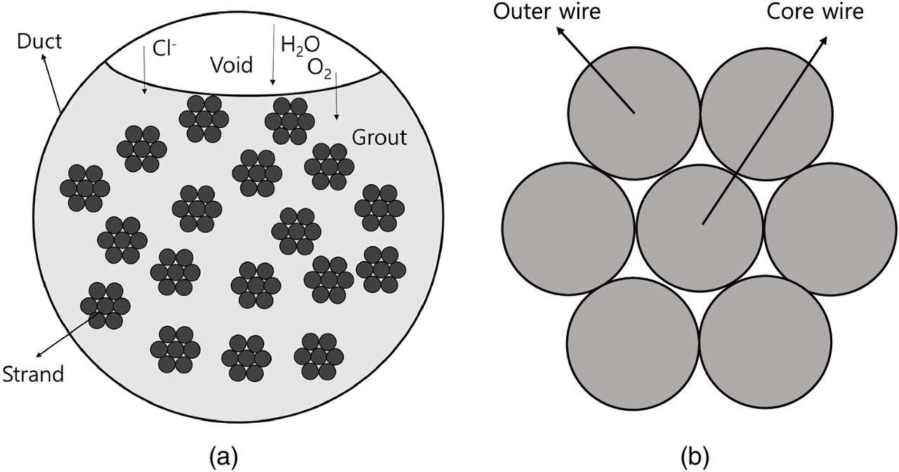
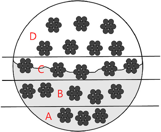
A void in the grout allows corrosion-promoting substances such as moisture, oxygen, and chloride to contact the strands, which may induce corrosion in the area. In fact, according to the samples of corroded strands obtained from the actual bridge (SMFMC 2017), most of the corrosion was found in the strands exposed to the void. Therefore, in many countries, the presence of void in the grouts is checked during safety inspections of PSC girder bridges. In addition, carbonation depth, water-cement ratio, and chloride content are often measured to investigate the corrosive environment. According to the Federal Highway Admininstration (FHWA) report (Lee and Zielske 2014), the farther the strand is located away from the void and the lower the water-cement ratio and chloride content are, the safer it is against corrosion. Thus, it is reasonable to classify the corrosive environment in terms of the distance between the strand and the void inside the duct. It is also noted that the guideline on yearly safety inspection in South Korea (KISTEC 2019) classifies the corrosive environment in terms of the existence of void and the carbonation depth. Accordingly, this paper classifies the corrosive environment of strands into the four categories as described in Table 1. Fig. 2 illustrates the layers of strands matching Categories A, B, C, and D listed in Table 1.
| Category | Definition | Level of corrosion risk |
|---|---|---|
| A | No void, carbonation depth | Very low |
| B | No void, carbonation depth | Low |
| C | Void, carbonation depth | Intermediate |
| D | Void, exposed strands, carbonation depth | High |
Furthermore, the threshold of chloride concentration, in Eq. (1), which is the criterion regarding the occurrence of corrosion, should be determined differently for each category of the corrosive environment. In order to determine , several studies were carried out using experimental corrosion data from laboratories and corrosion samples from actual PSC girder bridges. Virmani and Ghasemi (2012) reviewed these studies to identify common characteristics of corroded steel strands as follows: (1) the bleeding water accumulates during grouting process; (2) corrosion initiates where the void exists in grout; (3) carbonated local area exists; (4) high relative humidity and moisture accelerate corrosion propagation; and (5) once corrosion initiates, corrosion can propagate rapidly because of high chloride concentration, presence of moisture, water, and high humidity. However, there is no well-established formula for the threshold of chloride concentration that can analytically consider the effects of environment, e.g., pH, temperature, humidity, and moisture, even though these variables greatly affect corrosion. Therefore, it is inevitable that the reference values for suggested by many researchers have great variability.
To address the variability, this paper models as a random variable that is based on the range values suggested in the literature and the guidelines of the current practice of structure safety inspection in South Korea. Currently, the values of from the guidelines are expressed as the total chloride content mass per unit volume . Conversely, Glass and Buenfield (1997) suggested that the best way to express the chloride threshold value is using the chloride content percentage of weight of cement. Accordingly, the total chloride content mass is divided into (mass per unit volume of cement) to determine the values of with a unit of percent of weight of cement. The maximum threshold value in Category A, the safest category against corrosion, is determined as 1.5% of weight of cement, which represents the best field conditions with high-quality grout containing no void or moisture (Virmani and Ghasemi 2012). Table 2 shows the ranges of the chloride concentration thresholds introduced for the four categories.
| Category | Threshold of chloride concentration (% of weight of cement) | Corrosion current density ( |
|---|---|---|
| A | 0.4–1.5 | 0.01–0.1 |
| B | 0.19–0.4 | 0.1–0.5 |
| C | 0.1–0.19 | 0.5–1.0 |
| D | 0.023–0.1 | 1.0–2.0 |
Lastly, the corrosion current density in Eq. (2), related to the corrosion propagation rate, also depends on the corrosive environment. The value of can be measured by the linear polarization resistance (LPR) technique, and the criteria of the corrosion current density are often presented for four conditions of corrosive environment: negligible, low, moderate, and high (Song and Saraswathy 2007; Lee and Zielske 2014). Based on the criteria, this paper determines the range of corrosion current density for the four categories as shown in Table 2.
Material Model of Corroded Strands
To reflect the actual behavior of corroded strands of PSC box girder bridges, this paper employs the stress-strain material model by Jeon et al. (2019). The model was developed based on corrosion inspection and tensile strength tests of a total of 16 seven-wire strands samples taken from the Jeongneungcheon overpass bridge which experienced the failures of external tendons. The original (not corroded) seven-wire strand has a nominal cross-sectional area of , and a nominal diameter of 15.2 mm, while the nominal radius of outer wires and core wire are 2.6 and 2.5 mm, respectively. This is one of the most widely used strand types of PSC box girder bridges in Korea. The material model covers three corrosion types defined in terms of the corrosion shape of the wire. The section loss in each wire is calculated using the maximum pit depth and radius of the wire [more details available in Jeon et al. (2019)]. The stress-strain relationship was described by a bilinear model whose parameters are defined as follows based on the regression analysis:where and = ultimate stress and strain of a corroded strand, respectively; = yield stress; = maximum pit depth; = section loss ratio; and , and are the model coefficients described in Table 3.
(3)
(4)
(5)
| Type | |||||||
|---|---|---|---|---|---|---|---|
| Type 1 | 1,748.0 | 0.0754 | 0.0025 | ||||
| Type 2 | 1,801.6 | 0.0754 | 0.0045 | ||||
| Type 3 | 1,752.7 | 9.54 | 0.0754 | 0.0045 |
Source: Data from Jeon et al. (2019).
Estimation of Traffic Load Effects and Flexural Strength of PSC Box Girder
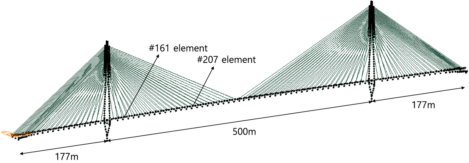
Cross Sections of the Example Bridge (Hwayang-Jobal Bridge)
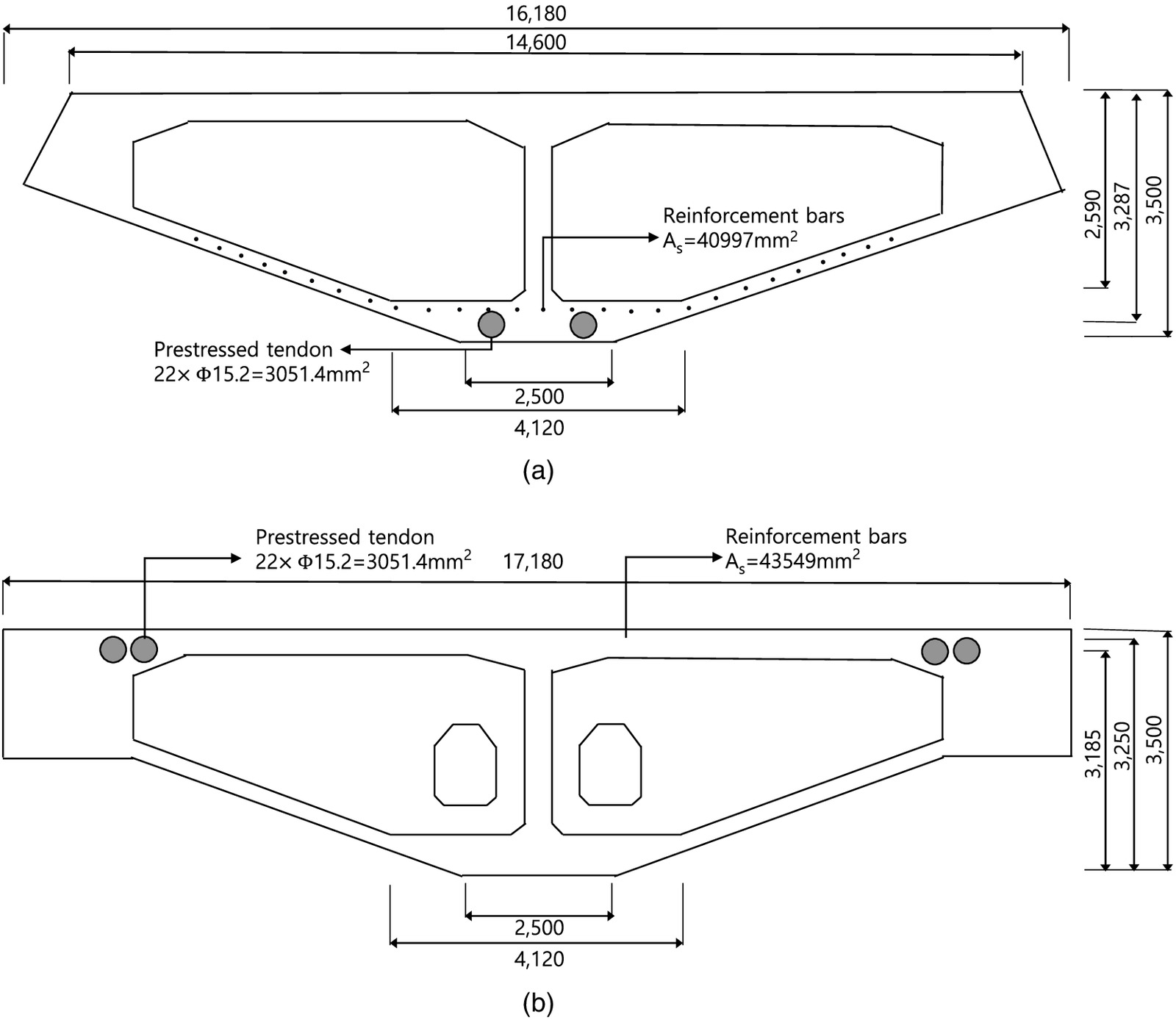
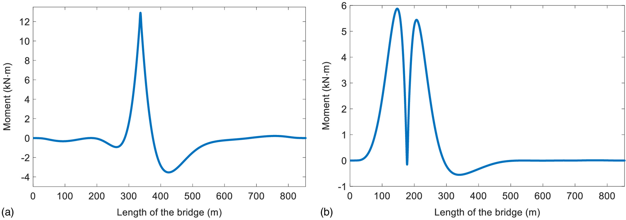
In order to demonstrate the time-dependent reliability analysis based on the estimation of traffic load effects and flexural strength, the Hwayang-Jobal Bridge is selected as the example bridge. This cable-stayed bridge connecting Yeosu and Goheung in South Korea has two lanes and a total length of 854 m and a main span of 500 m. The type of a stiffened girder of this bridge is post-tensioned concrete (PSC) box girder with external and internal tendons, each of which consists of 22 steel strands and a duct. A finite-element model was constructed based on the structural calculation document of the bridge to estimate traffic load effects (the bending moment of the girder) and the flexural strength of each cross section. The cross sections with the lowest level of reliability with regards to the positive moment and the negative moment are selected respectively. Fig. 3 shows the constructed finite-element model and the locations of selected cross sections (#207 element for the positive moment, and #161 element for the negative moment). Figs. 4(a and b) show the selected cross sections for the positive and negative moment. The positive moment cross section has two external tendons while the negative moment cross section has four internal tendons. The next section presents how the traffic load effects and the flexural strength are estimated for these cross sections.
Calculation of Traffic Load Effects Using Traffic Environment Information
To estimate the traffic load effects based on the actual traffic environment of Hwayang-Jobal Bridge, this paper uses the WIM-based probabilistic model of bridge traffic loads (Kim and Song 2019) and the Bayesian updating methodology (Kim and Song 2021). First, appropriate values are set for the parameters of the traffic load model based on the traffic investigation and WIM data of the example bridge and surroundings. Next, the traffic flow is simulated for a desired period using the traffic load model. Then, the traffic load effects are computed using the influence lines of the structural members of interest. Lastly, the probabilistic distribution of the maximum traffic load effects during the service life of a bridge or the return period of a load level is obtained based on samples of the calculated traffic load effects and the extreme value theory.
To estimate the traffic load effects of the selected cross sections, the bending moment influence lines for the two cross sections are first obtained as shown in Fig. 5, and the traffic environment of Hwayang-Jobal Bridge is investigated. However, accumulated data related to the traffic environment over a long period of time are not available because of the short operation period of the bridge. Thus, this paper uses the traffic information of roads, which was obtained from the regular traffic investigation on the area around the example bridge, to approximate the actual traffic environment. Because the example bridge has a long span (a total length of 854 m), the maximum traffic load effect occurs under a congested traffic flow, i.e., where many vehicles exist on the bridge (Kim and Song 2019). Hence, the average speed under congestion and the occurrence frequency of the congestion state are necessary when simulating the traffic flow. The ratio of heavy vehicles such as large truck and trailer, which is an important variable affecting the maximum traffic load effect, is also needed. To obtain this information, the traffic environment of the example bridge is inferred based on its location. Because the bridge is located around many islands and tourist attractions, it is assumed that, on weekends, the traffic volume increases significantly, the ratio of heavy vehicles is low, and the ratio of passenger cars is high. Actually, a traffic volume measured during a weekend was 10,944 vehicles/day, which exceeded the design traffic volume of 7,142 vehicles/day. Using the measurement of traffic volume, the average speed under congestion is estimated indirectly through the volume delay function (VDF) as follows (Spiess 1990):where = standard travel time; is the travel time given the traffic volume; = capacity of road; = traffic volume; and and are the model parameters. As a result, the average speed under congestion is estimated as , and it is assumed that this level of congested traffic flow occurs for 2 h per weekend (104 h/year). The ratio of heavy vehicles is assumed to be 3% based on the traffic data from the surrounding of the bridge (MOLIT 2019). To consider the impact load, 25% impact load factor, which is specified in the Korean highway bridge design code (MOLIT 2015), is used in the paper.
(6)
Based on the assumed parameters of the traffic environment, 100 samples of 1-year maximum traffic load effect are calculated from the simulated traffic flow for 1 year. The 100-year maximum traffic load effects (corresponding to the estimated traffic load effect from the design code) are then calculated using extrapolation as shown in Table 4. The traffic load effects estimated from the initial traffic environment are smaller than those from the design code because the ratio of heavy vehicles is relatively low and severe traffic congestion does not occur frequently under the initial traffic environment.
| Traffic loading condition | Positive moment | Negative moment |
|---|---|---|
| Design code | 18,323.4 | 16,946.1 |
| Initial traffic environment | 12,446.2 | 13,494.5 |
| Changed traffic environment (100 years) | 19,219.1 | 22,542.7 |
Furthermore, the change of the traffic environment during the service life of the bridge is considered in this study through the following virtual scenario. It is assumed that, due to the industrialization of cities and the construction of many factories around Hwayang-Jobal Bridge in future, the demand for the volume of cargo transportation continues to increase, resulting in a growth of the ratio of heavy vehicles, and severe traffic congestion occurs more frequently on weekdays than on weekends. To reflect this change of traffic environment, it is assumed that the ratio of heavy vehicles and the frequency of congested traffic flow increase linearly, and the average congested speed decreases. Accordingly, after 100 years, the ratio of heavy vehicles is assumed to reach 35% based on the data from other roads experiencing many heavy vehicles in Korea. It is also assumed that the congestion occurs for 1 hour on each weekday (260 h/year) and the congested speed decreases to . Based on these assumptions, the traffic load effects for the changed traffic environment after 100 years are estimated as shown in Table 4. Note that both estimated traffic load effects (positive and negative moment) from the changed traffic environment increase and exceed those from the design code. The negative moment increases more significantly than the positive moment because of the shape of the influence line, as shown in Fig. 5. The influence line of the positive moment has a large area with the opposite sign of the moment (causing adverse traffic load effect against maximum traffic load effect). Conversely, the influence line of the negative moment has a relatively small area with the opposite sign of the moment.
Calculation of Flexural Strength Considering Corroded Strands
For efficient evaluation of reliability, which is comparable with that in the design code, this paper calculates the flexural strength in the same way as the code. An iterative method to satisfy the force equilibrium and the strain compatibility condition specified in the current Korean highway bridge design code (MOLIT 2015) is employed. Additionally, the material model for corroded strands described in the section “Material Model of Corroded Strands” is introduced when calculating the flexural strength of the girder with strand corrosion considered. The other material models used in the paper are as follows. For concrete and reinforcement bars, the parabolic-rectangular model and the elastic–perfectly plastic model provided in the design code (MOLIT 2015) are used, respectively. A seven-wire corrosion-free strand, in which each of the six outer wires has a radius of 2.6 mm and the core wire has a radius of 2.5 mm, has a nominal cross-sectional area of , and a nominal diameter of 15.2 mm. The strand, represented by the bilinear model with the material properties in Table 5 (Jeon et al. 2019), is employed.
| Elastic modulus (MPa) | Yield strength (MPa) | Yield strain | Ultimate strength (MPa) | Ultimate strain |
|---|---|---|---|---|
| 195,000 | 1,628 | 0.0083 | 1,865 | 0.075 |
Before computing the flexural strength, the girder of the example bridge is subjected to both bending moments and axial forces, unlike the girder of a general bridge, which is subjected to bending moments only. Therefore, in this case, the effect of axial force on flexural strength is considered through the P-M interaction diagram. For example, columns are generally designed using the P-M diagram to consider the simultaneous actions of axial force and bending moment. However, the axial force acting on the target cross section of the example bridge ( for #161 element), is less than about 20% of the pure axial strength of the cross section, which is the -intercept of P-M diagram ( for #161 element). Furthermore, because the girder is a flexural member, the effect of the applied bending moment is significantly larger than that of the actual axial force. Therefore, according to the actual structural calculation document made for the example bridge, engineers judged that the design criterion for axial strength is automatically satisfied even if the cross section is designed by considering only the flexural strength. Accordingly, this study also calculates flexural strengths without considering the action of axial force in order to calculate the reliability, which is comparable to the reliability estimated from the design stage and for efficient computation of reliability. However, in the future, it is necessary to quantitatively analyze the effect of the axial force on the flexural strength through methods such as P-M interaction diagram for a more accurate reliability evaluation.
According to the design code, when starting the calculation of flexural strength with the iterative method, the maximum strain of the compression part of the concrete is assumed as the ultimate compressive strain of concrete, i.e., around 0.003, to induce ductile failure. Next, assume the depth of the neutral axis, and then the strain of the reinforcement bars and strands are obtained bywhere and = strains of reinforced bars and strands, respectively; = ultimate compressive strain of concrete; and = distances from the top of the concrete compression part to the centroid of the rebars and the strands, respectively; = depth of neutral axis; = effective prestress; and = elastic modulus of the strand. In the case of PSC bridges, unlike general reinforced concrete bridges, prestressing force is applied in advance, so a term containing is included in Eq. (8). The loss of the prestressing force occurs instantaneously and gradually over time due to the elastic deformation of concrete, the relaxation of the strand, the anchorage slip. Therefore, the loss of prestressing force should be considered.
(7)
(8)
A ratio defined by Youn (2013) is considered as follows:which is defined as the distance between the neutral axis and the top surface of the concrete under compression to the distance between the neutral axis and the centroid of the PS strands. For PSC box girder bridges, this ratio is usually high because the width of the compression part is relatively wide, as shown in Fig. 4 (Youn 2013). When the ratio is larger than 4 in a flexural member, the initial strain caused by the effective prestress [the second term including in Eq. (8)] is much smaller than that caused by ultimate loads [the first term including in Eq. (8)]. Thus, the effects of the loss of prestressing force on the flexural strength of the PSC box girder is negligible (Youn 2013). The ratio in Eq. (9) for the selected cross sections of the girder of the example bridge is also greater than 4. Therefore, for efficient estimation of flexural strength, this paper employs an assumption that the prestressing force is reduced by 30% instead of accurately calculating the prestressing force loss. Because is significantly small due to the wide width of the compression part, the failure of the strand sometimes occurs before the maximum strain of the compression part of the concrete reaches . This case violates the assumption in the design code introduced to induce ductile failure, and thus may lead to a convergence problem when calculating the flexural strength. This paper addresses this issue by gradually reducing the assumed maximum strain of the compression part of concrete when a convergence problem occurs.
(9)
Once corrosion occurs in steel strands, the corroded wires no longer behave linearly. Therefore, in Eq. (8) cannot represent the strain caused by the effective prestressing force. In this case, should be obtained differently by calculating the initial strain caused by the prestressing force from corroded strands, that is
(10)
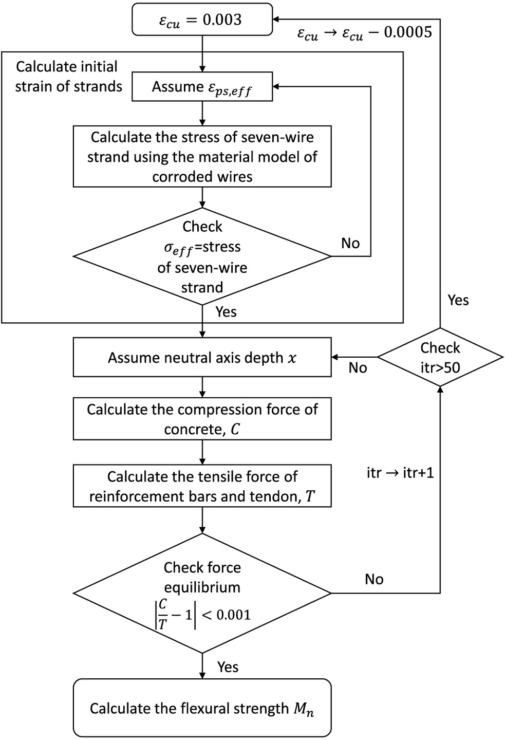
To obtain by considering the nonlinear behavior of the corroded wire, this paper uses an assumption that the strain is proportional to the distance from the neutral axis even if corrosion occurs (Jeon et al. 2019). Then, initial strain is calculated iteratively through the stress redistribution among seven wires while maintaining the prestressing force of the strand. Next, using the strain of strands calculated by Eq. (10), the tensile force of the strands is calculated using the material model of corroded strands. The tensile force of the reinforcing bar and the compression force of concrete are also calculated based on the estimated strain and the corresponding material models. Finally, the force equilibrium condition is checked using the calculated tensile force and compression force, and if the equilibrium is satisfied, the iteration is terminated to determine the flexural strength. Additionally, because corrosion primarily occurs in outer wires, it is conservatively assumed that corrosion occurred in six outer wires excluding the core wire among the seven-wire strand. Fig. 6 is the flow chart describing the iterative method to calculate the flexural strength.
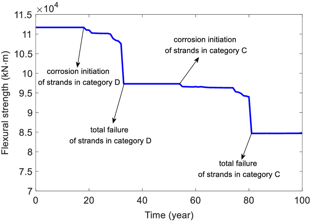
Using Eqs. (1) and (2), and the iterative method described previously, the flexural strength of the girder during the service life is calculated as follows. First, each strand is assigned to one of the categories of corrosive environment in Table 1. Next, the corrosion initiation time for the stands in the same category is calculated using Eq. (1). Then, the strands with and without corrosion are distinguished using the calculated corrosion initiation time and the relevant parameters for each strand. For the strand without corrosion, a material model for strands without corrosion is used. For the strands with corrosion, the maximum pit depth for the strands in the same category is calculated using Eq. (2), and the depth is used to obtain the section loss ratio of wires in the strand [see additional details in Jeon et al. (2019)]. Subsequently, the material model of corroded strands in the section “Material Model of Corroded Strands” is determined through the section loss ratio. Finally, the flexural strength is calculated by the iterative method based on the material models defined for strands. For example, Fig. 7 shows the result of calculated flexural strength over 100 years for the cross section of the negative moment using certain fixed values for random variables. Among 22 strands in each tendon, 5, 5, 6, and 6 strands are classified into Categories A, B, C, and D, respectively. Strands in Categories A and B do not experience corrosion, while corrosion initiated at the strands in Category D in the 18th year and total failure occured in the 33rd year. Strands in Category C suffered corrosion from the 54th year and totally failed in the 81st year.
Time-Dependent Reliability Assessment
Limit State Function and Random Variables
This section describes the limit state function and random variables used in the time-dependent reliability assessment of the example bridge over its service life. The Korean highway bridge design codes (MOLIT 2015) define ultimate, serviceability, fatigue, and extreme event limit states. Among them, the Ultimate limit state 1 (ULS 1), which is a basic load combination that mainly considers the traffic flow (without wind load), is selected for the time-dependent reliability assessment in this paper. The limit state function of ULS 1 is given aswhere = flexural strength of the girder; and = bending moment determined by the dead load of structural members and nonstructural attachments (denoted by ), and the dead load of wearing surfaces and utilities (denoted by ). is the bending moment from the prestressing force applied by the cables and tendons; and is the bending moment from the traffic loads.
(11)
It might seem inappropriate to use traffic load effects estimated by influence lines from a linear structural analysis because the behavior of the bridge is usually in a nonlinear range when exceeding the ultimate limit state. However, note that existing design codes and many previous studies employ such an approach as an approximation because nonlinear structural analysis may require exceedingly high computational cost, especially when a sampling method is used for reliability calculations. Therefore, this study adopts the approximate method for efficiency, while leaving its impact on accuracy as a future research topic.
To perform reliability analysis, statistical properties of the random variables, which represent the uncertainties in material properties, corrosive environment, and loads in the limit state function, are investigated through the literature. As a result, the statistical properties of the 22 random variables are summarized as shown in Table 6. The nominal and mean values for material properties such as concrete strength and ultimate strength of strands are determined from the structural calculation document. The statistical properties of corrosion-related variables used in Eqs. (1) and (2) are determined based on the literature and guidelines of the current practice of structure safety inspection. As for the random variable , a bounded range is assigned to representing each of the four categories of corrosive environment in Table 2. In addition, has large variabilities because it is significantly affected by many factors such as pH, temperature, and humidity (Virmani and Ghasemi 2012) while there exist no well-established methods or equations to consider these factors. Thus, uniform distribution is used to describe in this paper instead of the normal or lognormal distributions that were generally used in previous studies. The parameters of uniform distribution for and are determined by their feasible ranges for each category of the corrosive environment described in Table 2.
| Variable | Property | Parameter | Distribution | Reference |
|---|---|---|---|---|
| Concrete strength | Nominal = 45 MPa, | Lognormal | Kim (2018) | |
| Bias = 1.158, COV = 0.095 | ||||
| Ultimate strength of prestressing wire | Mean = 1,865 MPa, | Normal | Lee et al. (2020) | |
| COV = 0.02 | ||||
| Yield strength of reinforcement bar | Nominal = 400 MPa, | Lognormal | Kim (2018) | |
| Bias = 1.15, COV = 0.08 | ||||
| Elastic modulus | Nominal = 200,000 MPa, | Lognormal | Lee (2019) | |
| Bias = 1.0, COV = 0.06 | ||||
| Concrete cover | Mean = 21 mm, COV = 0.05 | Normal | Nguyen et al. (2013) | |
| Diffusion coefficient | Mean = 0.631 , COV = 0.2 | Lognormal | Val and Trapper (2008) | |
| Chloride concentration threshold (A) | [0.4, 1.5]% of cement weight | Uniform | KISTEC (2019), Virmani and Ghasemi (2012) | |
| Chloride concentration threshold (B) | [0.19, 0.4]% of cement weight | Uniform | KISTEC (2019), Virmani and Ghasemi (2012) | |
| Chloride concentration threshold (C) | [0.1, 0.19]% of cement weight | Uniform | KISTEC (2019), Virmani and Ghasemi (2012) | |
| Chloride concentration threshold (D) | [0.023,0.1]% of cement weight | Uniform | KISTEC (2019), Virmani and Ghasemi (2012) | |
| Corrosion current density (A) | [0.01, 0.1] | Uniform | KISTEC (2019), Song and Saraswathy (2007) | |
| Corrosion current density (B) | [0.1, 0.5] | Uniform | KISTEC (2019), Song and Saraswathy (2007) | |
| Corrosion current density (C) | [0.5, 1.0] | Uniform | KISTEC (2019), Song and Saraswathy (2007) | |
| Corrosion current density (D) | [1.0, 2.0] | Uniform | KISTEC (2019), Song and Saraswathy (2007) | |
| Penetration ratio | [4, 6] | Uniform | El-Maaddawy and Soudki (2007) | |
| Sectional loss area | Bias = 1.0, COV = 0.05 | Lognormal | Lee et al. (2020) | |
| Professional factor for strength | Mean = 1.0, COV = 0.06 | Lognormal | Nowak and Szerszen (2003) | |
| Dead load of structural members | Bias = 1.03, COV = 0.08 | Normal | Nowak (1999) | |
| Dead load (2nd) | Bias = 1.00, COV = 0.25 | Normal | Nowak (1999) | |
| Prestress force | Bias = 1.0, COV = 0.06 | Normal | Nowak (1999) | |
| Live load | Estimated parameters | GEV | Kim and Song (2019) | |
| Influence factor for live load | Mean = 1.0, COV = 0.06 | Normal | Nowak (1999) |
The random variable sla represents the uncertainty in estimating the sectional loss area through the maximum pit depth (Lee et al. 2020). The professional factor prf is a coefficient describing the uncertainty from the difference between the strength analysis model and the actual strengths of structural members (Ellingwood 1980). This paper adopts the statistical properties of prf suggested by Nowak and Szerszen (2003). The nominal values of and are estimated based on the structural calculation document and their statistical properties are determined based on the literature.
The uncertainty in the traffic load effect is generally considered through the following equation (Ellingwood 1980):where = random variable of the traffic load effect; = modeling parameter that considers the uncertainty caused by idealizing the actual traffic load as a live load model in the design code; = influence factor representing the uncertainty arising from the structural analysis to calculate the traffic load effect; and = traffic load (axle weight, total weight of the vehicle) acting on the bridge. Because the traffic load effect is calculated by direct simulation of the traffic flow with the influence line in this paper, can be described as a random variable following the generalized extreme value (GEV) distribution based on the extreme value theory. The is not included as a random variable because a live load model of the design code is not used in this study when estimating the traffic load effects. The influence factor (Nowak 1999) is selected as a random variable as shown in Table 6.
(12)
Computation of Time-Dependent Reliability
Time-dependent reliability assessment aims to evaluate the reliability of an engineering system over its service life. Many researchers have studied how to efficiently calculate time-dependent reliability and have applied various methods to actual structures (Andrieu-Renaud et al. 2004; Li et al. 2015; Wang et al. 2017; Qian et al. 2020; Straub et al. 2020). According to Gong and Frangopol (2019), reliability methods that cover external loadings and the deteriorating process can be classified into three categories: the Poisson process load method (Yang et al. 2017), the extreme value-based method (Wang and Wang 2012), and the first-order reliability method (FORM)-based outcrossing rate method (Andrieu-Renaud et al. 2004). Among these categories, the extreme value-based method is employed because in the case of ULS1, the strength and the load process can be modeled independently and various loads can be grouped into time-invariant loads and time-variant loads, which can be approximated by maximum loads. Further details of the computation process are provided below in this section. In addition, for convenient and efficient computation, the service life is often discretized to a series of time intervals. The time-variant reliability problem is then transformed into a time-invariant reliability problem that can be solved through a system reliability method for the series system. This approach can be applied to the general structural systems regardless of structural types (Melchers 1999). Therefore, in this paper, time-dependent reliability for the example bridge is computed by discretizing service life into certain intervals to apply the system reliability method for the series system.
A limit state function defined by two groups of random variables describing strengths and loads, respectively, e.g., ULS 1, can be described as (Straub et al. 2020)where = structural strength affected by the corrosion process; = vector of random variables related to the strength and corrosion; and = load effect determined by the combination of the loads, i.e., in Eq. (11). The service life is discretized into a series of time intervals indexed by . The th interval corresponds to the time duration . The probability of the interval failure event is formulated aswhere = time-varying load vector during the time interval ; and the time-varying strength during the time interval is approximated by the strength at the end point, i.e., . Note that the approximation made in Eq. (14) holds when the service life is discretized into a large number of intervals. To reduce the computational cost, a further approximation is made as follows by replacing the load vector by the maximum loads over the interval, through an extreme value analysis:
(13)
(14)
(15)
As a result, the failure probability during a given interval can be computed by a time-invariant reliability analysis. Note that, in the case of ULS 1, the temporal variability of the traffic load is significantly larger than those in the other loads. Therefore, the load vector can be split into the time-variant load , and the group of time-invariant loads . As a result, the interval failure probability can be efficiently evaluated as (Straub et al. 2020)where denotes the maximum live load during the time interval . Without losing general applicability, this paper adopts subset simulation (Au and Beck 2001) to obtain interval failure probability in Eq. (16) because the method facilitates efficient calculation of the probability of a rare event in a high dimensional problem. In this paper, to calculate interval failure probability through subset simulation, samples and conditional probability are used for each intermediate subset. The adaptive conditional sampling method is used as the Markov chain Monte Carlo (MCMC) sampling method to obtain samples of each subset. For more details of the used sampling method, the reader is referred to Papaioannou et al. (2015).
(16)
Next, the failure of the structure up to time (or up to the endpoint of the interval ) can be described by the union of the interval failures, that is
(17)
In order to efficiently evaluate the series system failure probability ], upper and lower bounds using unicomponent probabilities can be computed as (Boole 1854)
(18)
In addition, the following narrower bound, based on the assumption that interval failure events are independent of each other, is often used (Val et al. 2000; Schneider et al. 2017):
(19)
However, these bounds are often too wide to be useful. For narrower bounds, the information regarding the statistical dependence between the interval failure events need to be incorporated (Song and Der Kiureghian 2003).
Among a variety of system reliability methods (Song et al. 2021) that were developed to compute the series system failure probability, this study adopts the approach by Straub et al. (2020) in which the FORM approximation is estimated by a sampling method. This approach was developed to cover the same kind of problems as ULS1, which is used as the limit state in this paper. In addition, this approach can update the time-dependent reliability using inspection and monitoring data and can reduce the computational cost. In this approach, is evaluated by the FORM approximation (Hohenbichler and Rackwitz 1982), that iswhere is the multivariate standard normal cumulative distribution function (CDF) at vector which is the set of the reliability indices for the interval failure events . The elements of the correlation coefficient matrix are obtained bywhere = correlation coefficient between the failures of the interval and ; and and = negative normalized gradient vectors (Der Kiureghian 2005) from FORM analysis of the corresponding intervals. Straub et al. (2020) proposed to estimate them using a sampling-based method, that iswhere is the th sample of standard normal vector in the failure domain; and = total number of the samples. Refer to Straub et al. (2020) for more details.
(20)
(21)
(22)
Furthermore, note that the uncertainties in the random variables related to corrosion and traffic environment are naturally large due to many uncertain factors in the surroundings. Therefore, it is desirable to update the reliability based on data and information gained during the lifespan of the bridge. Introducing an event that representing the data measured up to time , the failure probability can be updated to the conditional probability
(23)
The data measurement at time implies that the structure must have survived up to time . Therefore, the failure probability for should be updated accordingly as (Straub et al. 2020)
(24)
Both conditional probabilities and are calculated by Eq. (23) after changing the distribution parameters of the measured variables accordingly.
Numerical Examples
Time-Dependent Reliability Prediction Considering Traffic Environment and Corrosion of Strands
In the first numerical example, time-dependent reliability of the PSC box girder of the Hwang-Jobal bridge is evaluated by applying the proposed framework. In order to investigate the influences of the traffic load and corrosion on time-dependent reliability, three cases are investigated: (1) considering changes in traffic load only, (2) considering corrosion of the strand only, and (3) considering both. Besides, using the four categories of corrosive environment for the strand defined in Table 1, the 22 strands existing in each tendon are classified into Categories A, B, C, and D. The time-dependent reliability over the 100-year service life is evaluated for three scenarios of corrosion environment defined in terms of the number of strands belonging to the four categories: (1) vulnerable to corrosion (A: 0, B: 0, C: 11, D: 11); (2) moderate (A: 5, B: 5, C: 6, D: 6); and (3) robust (A: 11, B: 11, C: 0, D: 0). It is assumed that the cross-sectional areas of reinforcement bars decrease by 0.5% per year from the 20th year due to corrosion, and is set as 0.15% of the cement weight.
To calculate the probability of the interval failure , this paper discretizes the service life of the bridge (100 years) into 5-year-long intervals. For each interval, subset simulation is performed using the assumed conditions regarding corrosive environment and traffic, and the random variables summarized in Table 6. Next, is computed using the FORM approximation along with sampling to compute the correlation coefficients, as described in the previous subsection. However, if the interval failure probability is lower than about (reliability index is greater than around 7), the CDF of the multivariate standard normal distribution in Eq. (20) cannot be precisely evaluated even if a state-of-the-art algorithm (Botev 2017) is used. In this case, the upper and lower bounds on are evaluated by Eq. (18) instead, and then converted to the corresponding reliability index. Since the bound widths of time-dependent reliability in the example are highly narrow, for a clear presentation, the lower bound of reliability index is used as the result of time-dependent reliability analysis as shown in Figs. 8 and 9.
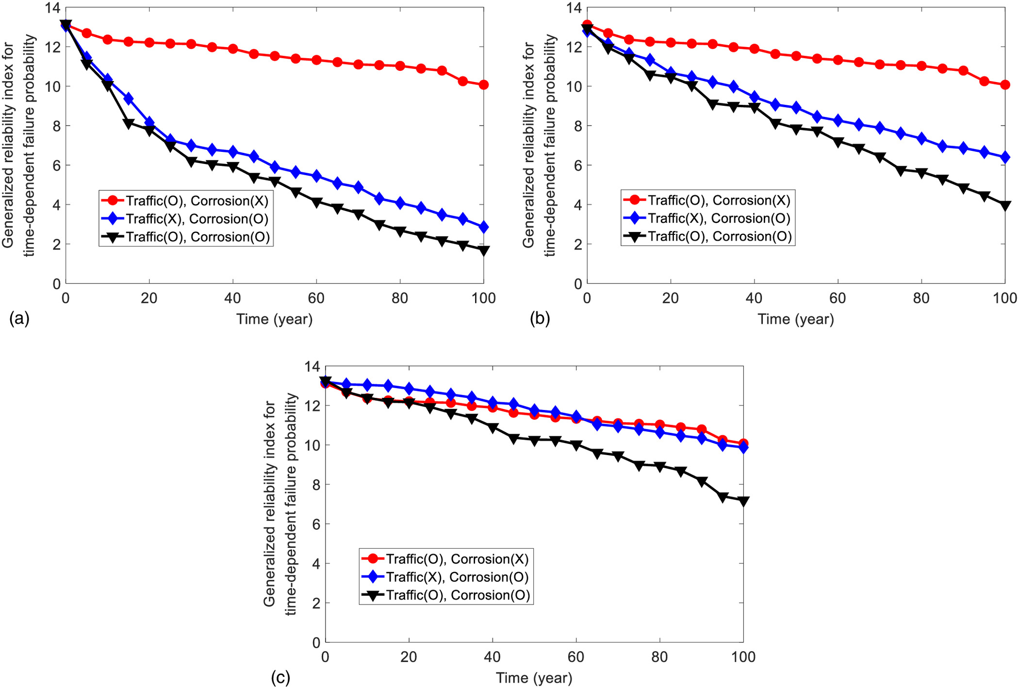
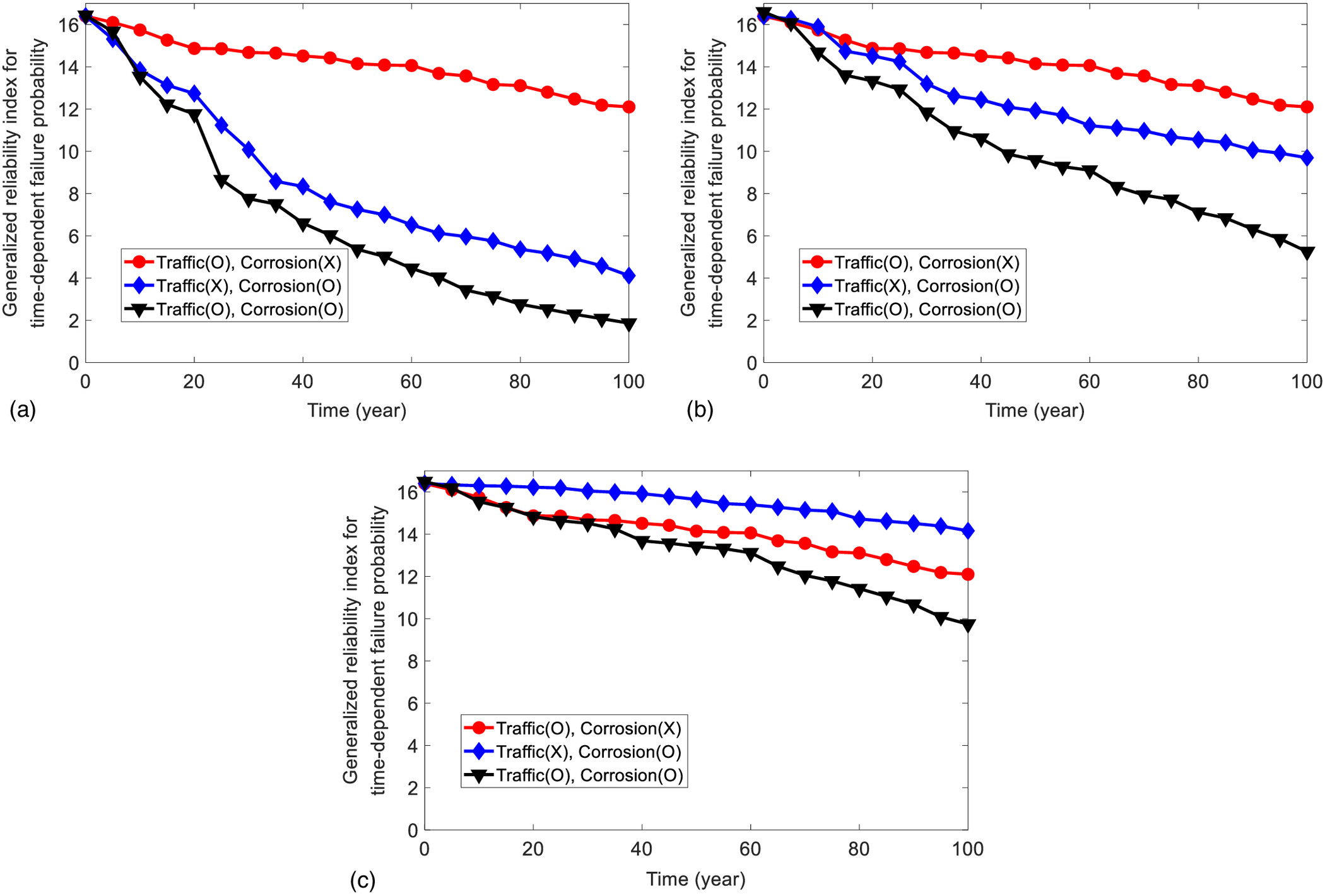
Before analyzing the results, note that the evaluated reliability index is significantly higher than the general range of bridge reliability index, around 3–4. This is because, first, the evaluated time-dependent reliability at a certain time point in this paper is derived from the failure probability over the time period not the whole service life . Therefore, the evaluated time-dependent reliability in the early time can be higher than the general bridge reliability index because of the short time duration. In order to clarify the meaning of the evaluated time-dependent reliability, it is expressed as the generalized reliability index for time-dependent failure probability in this paper. Second, this paper uses the actual information of the bridge specified in the structural calculation document, which might be the results of conservative bridge design. In practice, the factored strength is quite higher than factored loads for ULS1 in the structural calculation document of the example bridge. Third, as a result of accurate estimation of traffic load effects and flexural strengths, coefficient of variation (COV) of variables related to traffic loads and flexural strengths used in the examples are significantly smaller than that of traffic loads and strength used in bridge design codes. Fourth, the example bridge is a cable-stayed bridge with PSC box girder, which has a higher level of redundancy than a general PSC box girder bridge. Furthermore, the reliability is evaluated for just Ultimate limit state 1 in this paper; thus, if the reliability is evaluated by considering other limit states, a lower reliability index can be derived.
The results show that when the structure is vulnerable to corrosion, the effect of corrosion of the strand on reliability is much greater than that of traffic loads in both cross sections of the positive and negative moment. For the second case in which the corrosive environment is moderate, corrosion of strands still has a greater effect than traffic loads in both cross sections. However, in the third case (robust to the corrosion), the effects of corrosion and traffic loads on reliability of the cross section of the positive moment become similar while traffic loads have a greater effect on reliability than corrosion in the cross section of the negative moment. This result implies that the effect of the traffic load on the reliability in the cross section of the negative moment is greater than in the cross section of the positive moment. The traffic load effects increase more over time in the cross section of the negative moment than in the cross section of the positive moment due to the difference in the shape of influence lines as explained in the section “Calculation of Traffic Load Effects Using Traffic Environment Information.”
Updating Effects of Inspection Data on the Time-Dependent Reliability Predictions
To investigate updating effects of the measured data and information regarding the random strengths and loads on the time-dependent reliability, the prediction shown in Fig. 9(b) considering both components are updated by data and information that could be obtained through the current practice of structure safety inspection in relation to the corrosion of the strands in the PSC box girder bridge. The structure safety inspection guidelines of KISTEC (2019) in South Korea cover various tests regarding concrete compressive strength, chloride content, and acoustic emission to check the existence of voids in the grout, carbonation depth test, and corrosion current density. As a general procedure of inspections regarding corrosion in PSC box girder bridges, an acoustic emission test can be performed first to check the presence of the void, which is the main cause of tendon corrosion. If the void is identified, the chloride content and carbonation depth test can be conducted as the next step. These tests can update the initiation time of corrosion, but cannot directly detect the occurrence of corrosion. Therefore, if there is a strong belief that corrosion has occurred, the inside of the tendon can be directly examined through an endoscope (SMFMC 2017), and the maximum pit depth, corrosion type, and corrosion current density can be measured additionally.
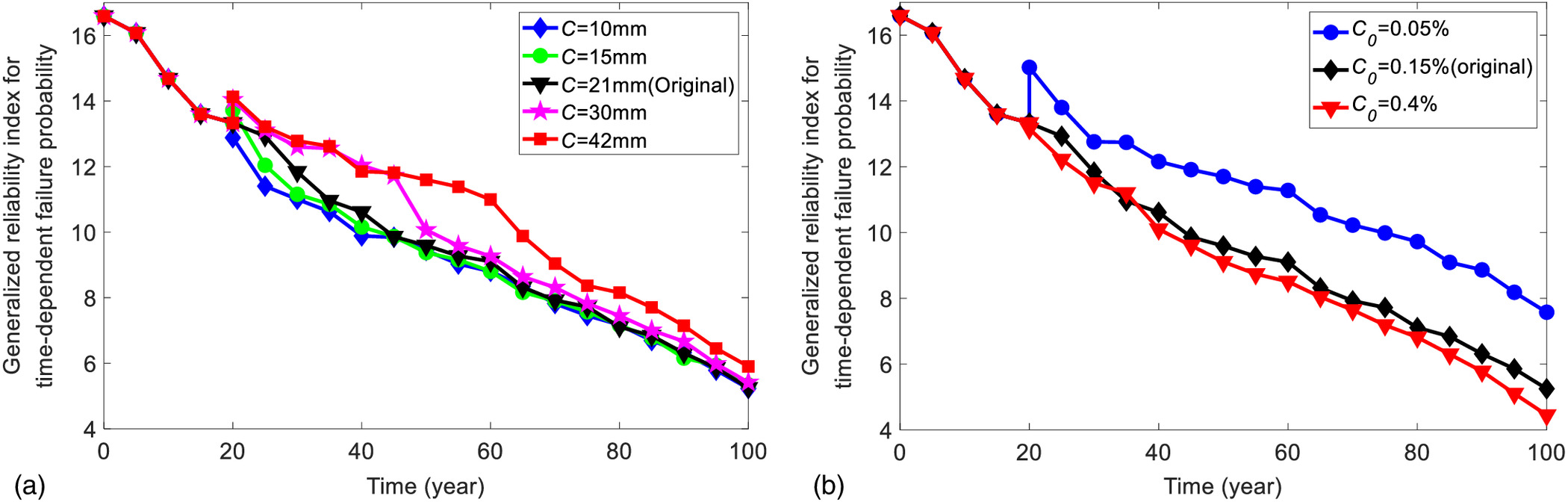
Before updating the time-dependent reliability using inspection data over the service life in the following sections, updating effects of measured data from each type of the aforementioned inspections on the reliability are investigated in advance. It is assumed that the data are measured in the 20th year. The time-dependent reliability after the 20th year is then updated using Eqs. (23) and (24) based on the measured data. As variables related to the corrosion initiation, the effects of the measured concrete cover thickness and chloride content on reliability are analyzed. In the meantime, as variables related to corrosion propagation, the effects of the maximum pit depth, corrosion current density, and corrosion type on reliability are also analyzed. As explained in the previous section, if the interval failure probability is extremely low, Eqs. (23) and (24) cannot be accurately evaluated. Therefore, the time-dependent reliability is conservatively updated in terms of the following upper bound:
(25)
Fig. 10 shows the time-dependent reliability updated based on the measured data of concrete cover thickness and chloride concentration at the surface. The results in Fig. 10 confirm that the thinner the concrete cover thickness is and the higher chloride concentration at the surface is, the earlier the corrosion initiates. This, in turn, causes the updated reliability index to decrease after the 20th year. However, the reliability updated using the measured data of concrete cover thickness becomes similar to the original one in the long term (after the 70th year) whereas the chloride concentration at the surface has a large effect on the reliability in the long term. The reason why the updated reliability differs greatly at the 100th year (end of service life) depending on the chloride concentration at the surface is that the number of corroded strands is determined by the chloride content.
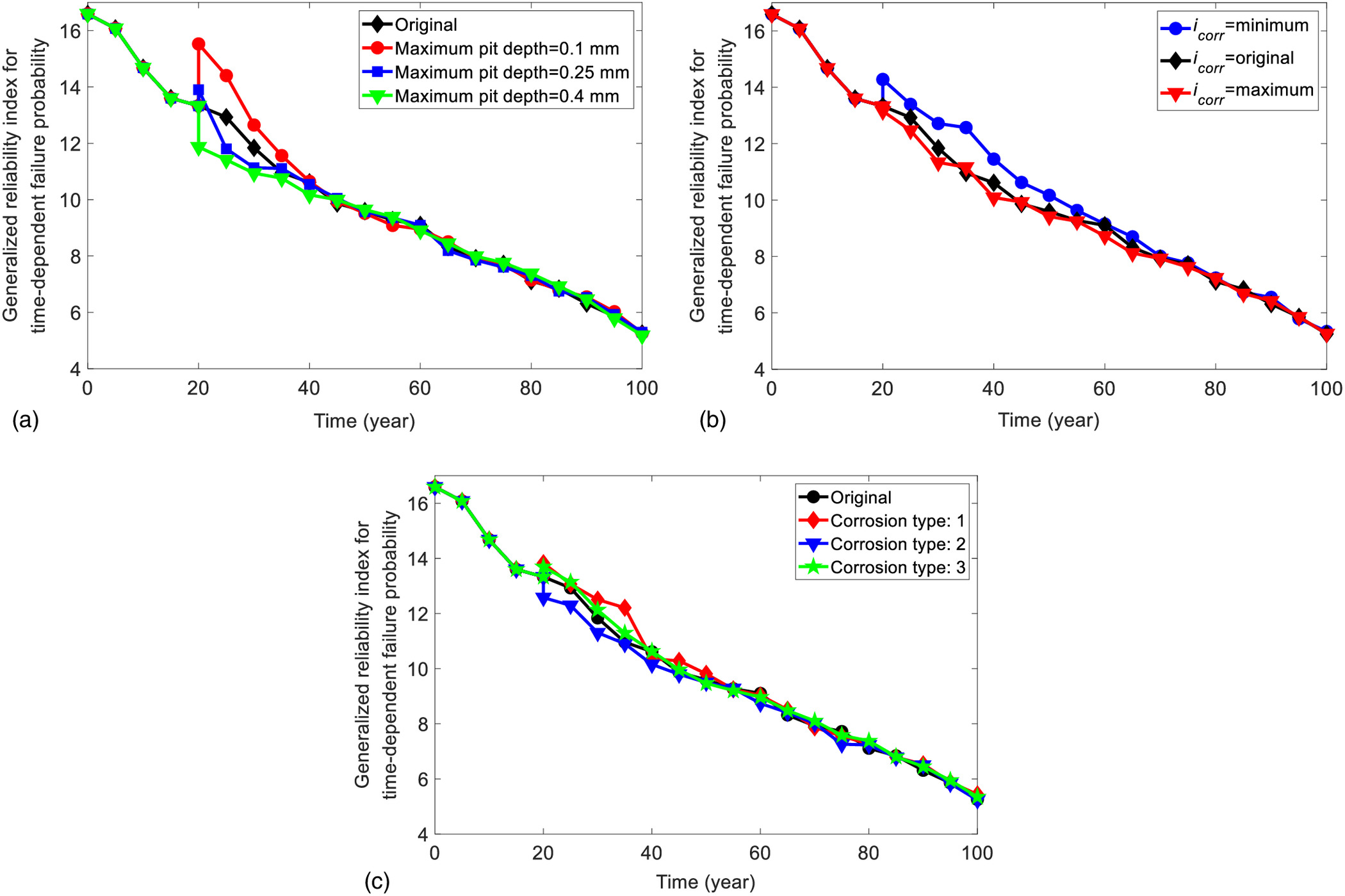
Conversely, Fig. 11 shows the time-dependent reliability updated based on the measured data of maximum pit depth, corrosion current density, and corrosion type. Fig. 11(a) shows that the change of reliability caused by the measurements of the maximum pit depth is quite large in the 20th year, i.e., the year when the data are measured. This is because the ultimate strain and strength of corroded strands are determined by the section loss area estimated using the maximum pit depth. However, regardless of the measurement of the maximum pit depth, 20 to 30 years after the inspection, the reliability of all three cases becomes similar to the original reliability. This is because once corrosion initiates, it proceeds rapidly, which makes most corroded strands in Categories C and D totally fail for all three cases. Fig. 11(b) shows that when the measured data of corrosion current density have the value of lower bound for each category defined in Table 2, the updated reliability becomes larger than the original reliability owing to the slow propagation of corrosion. However, after a certain time period passes, because most of the strands classified into vulnerable corrosive environments experience complete failures, the updated reliability become similar to the original reliability. As for the corrosion type, it is seen that the updated reliability of corrosion Type 2 decreases the most because corrosion Type 2 has the largest losses of section area when each corrosion type has the same maximum pit depth.
Maintenance Based on Time-Dependent Reliability Updating: Cross Section of Negative Moment
This section shows how the time-dependent reliability for the cross section of negative moment is updated using measured data and traffic scenario and can be used for the purpose of taking maintenance actions to assure target level of reliability.
Updating the Time-Dependent Reliability Using Measured Data and Traffic Scenario
The section “Updating Effects of Inspection Data on the Time-Dependent Reliability Predictions” shows that when the corrosive environment is vulnerable, corrosion can propagate rapidly within 20 to 30 years and may lead to the complete failure of the corroded strand. It was also reported in the literature that corrosion can propagate rapidly when the corrosive environment, e.g., the existence of voids, moisture penetration through air vents, low pH, high humidity, and high chloride content, is formed (Song and Saraswathy 2007; Virmani and Ghasemi 2012). Therefore, in the following updated example, it is assumed that the bridge is under a corrosive environment in which corrosion progresses rapidly for a short period of time (from the 30th to the 60th years). In addition, assumed measured data are introduced to describe the scenario of corrosion propagation and change of traffic environment. Every 6 years (30th, 36th, 42nd, 48th, and 54th year), a total of five monitoring and inspections are performed and the time-dependent reliability is updated using the measurements. Additionally, this paper checks whether the updated reliability satisfies the target reliability index in the Korean highway bridge design code (MOLIT 2015).
The target reliability index in this code is 3.72 for the defined service life of 100 years. However, the time period over which the time-dependent reliability is evaluated in the examples depends on the time point of assessment, ,not 100 years. Therefore, it is necessary to obtain the equivalent target generalized reliability index for the time period corresponding to 3.72 () for 100 years to check whether the updated reliability satisfies the target level of reliability. To this end, the mean annual failure probability corresponding to the reliability index of 3.72 for 100 years is first calculated by solving the following equation under the assumption that the failure events for 1-year intervals have the same probability and independent of each other:
(26)
As a result, the annual failure probability corresponding to the reliability index of 3.72 for 100 years is .Then, the corresponding target generalized reliability index for time-dependent failure probability for the time period is calculated by
(27)
The target generalized reliability index calculated by Eq. (27) is used in the examples to check whether the updated reliability satisfies the target level of reliability defined in the Korean highway bridge design code.
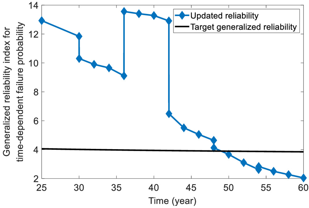
The following traffic scenario is considered in this example. Due to the urban development and industrialization of cities around the bridge from the 30th to 48th year, the ratio of heavy vehicles increases linearly from 10% to 35%. The frequency of congested traffic flow increases linearly from 120 h/year to 260 h/year while the average congested speed decreases from 30 km/h to 10 km/h. It is assumed that the changed parameters of the traffic environment are maintained until the 60th year. Next, the measured data and information from the inspection conducted every 6 years are created as follows. At the first inspection (30th year), the acoustic emission test confirms that there is no void in the grout, and the chloride content increases from 0.15% to 0.4%. At the second inspection (36th year), it is confirmed that there are voids in the grout, and the corrosive environment of the strands are classified by examining inside of the tendon using an endoscope. The 22 strands belong to the four categories as A:2, B:2, C:7, and D:11. However, corrosion of strands has not been found yet. At the third monitoring (42nd year), as a result of examining the inside of the tendon using an endoscope, corrosion of strands is found and the corrosion has progressed rapidly, so the maximum pit depth of the Categories C and D are measured as 0.12 and 0.25 mm, respectively. In addition, the corrosion current densities for Categories C and D are measured as maximum values and , respectively. At the fourth monitoring (48th year), the maximum pit depth of Category C increases to 0.2 mm, the maximum pit depth of Category D increases to 0.4 mm, and most of the corroded wires are classified to have corrosion Type 2. At the final monitoring (54th year), the measured corrosion current density decreases to the minimum values and for Categories C and D, respectively.
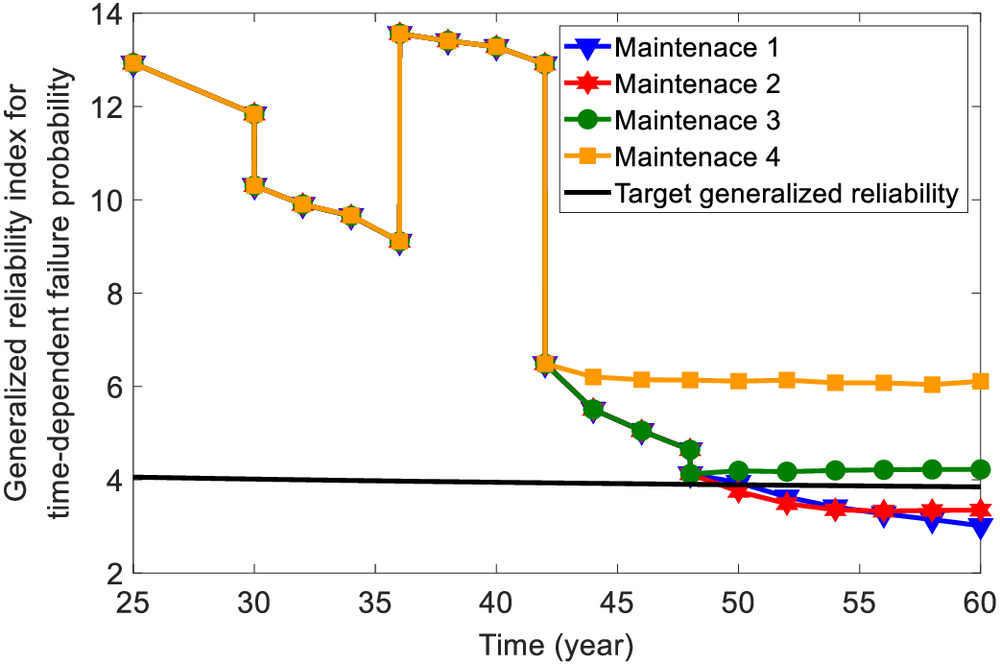
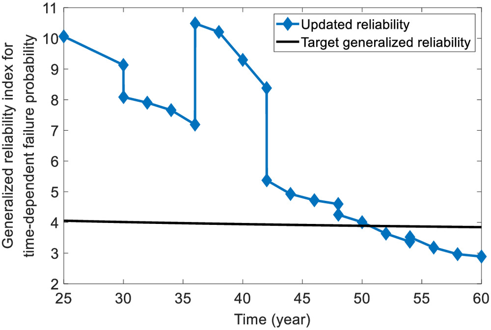
The results of the updates made with Eqs. (23) and (25) are based on the measured data explained previously are shown in Fig. 12. The reliability index decreased in the 30th year because the chloride content increased. In the 36th year, although the corrosive environment deteriorated, the reliability index increased because the corrosion was not observed. In the next inspection (42nd year), the reliability index decreased drastically because corrosion proceeded rapidly. In the 48th year, the reliability decreased because of the observed corrosion Type 2. In the final 54th year, the reliability slightly increased owing to the decreased measurement of corrosion current density. After the 48th year, it is confirmed that the updated time-dependent reliability becomes lower than the target generalized reliability index .
Maintenance Actions to Secure Target Reliability
To assure the safety of the example bridge, in this section several maintenance strategies are established, and the reliability after implementing maintenance actions is re-evaluated. When repair and maintenance actions are taken on a structure to secure target reliability, the state of the structure after a repair and maintenance action can be considered as statistically independent of the state prior to the repair action. Therefore, when calculating the reliability after the maintenance action, the reliability of the structure can be computed without consideration of the failure events prior to the maintenance action (Straub et al. 2020).
The first maintenance strategy considered in this section is to refill the grout and eliminate voids in the ducts in the 48th year to prevent further propagation of corrosion in the strands. The second strategy is to control the traffic environment by restricting the overweight vehicles (over 40 t) and reduce the traffic volume of the bridge through the construction of additional roads in the surroundings, thereby returning the ratio of heavy vehicles, the frequency of congestion, and the congested speed to those under the initial condition (30th year). The third strategy is to implement both the first and second strategies in the 48th year to deal with corrosive and traffic environments simultaneously. Finally, the fourth strategy is to implement both strategies in the 42nd year, earlier than the third strategy. Fig. 13 shows the results of updating time-dependent reliability after implementing the maintenance strategies. Although both the first and second strategies decrease reliability more slowly than the case of no maintenance decisions, i.e., the result in Fig. 12, their reliabilities are still under the target generalized reliability index. Conversely, when using the third strategy, which can improve corrosive and traffic environment simultaneously is implemented, the generalized reliability index can be maintained at a higher level than 4. When the fourth strategy that implements the maintenance action earlier is adopted, the generalized reliability index can be maintained at a higher level than 6.
Maintenance Based on Time-Dependent Reliability Updating: Cross Section of Positive Moment
This section shows how the time-dependent reliability for the cross section of positive moment is updated and can be used for the purpose of taking maintenance actions.
Updating the Time-Dependent Reliability Using Measured Data and Traffic Scenario
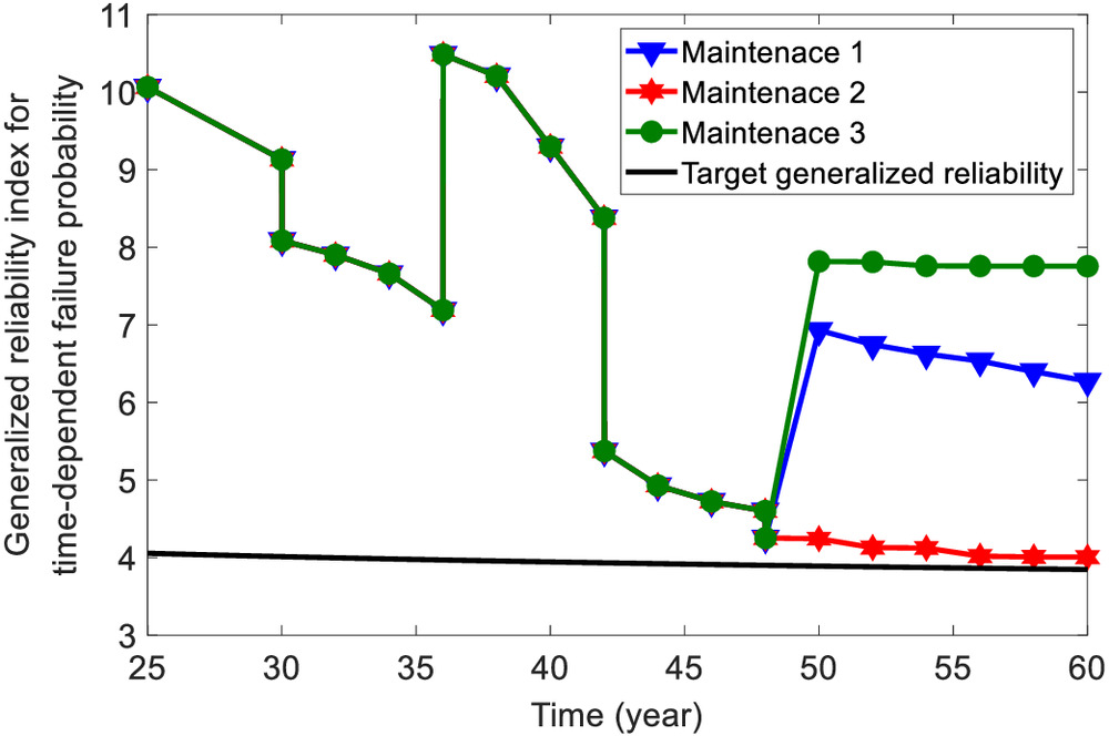
In the example of updating reliability of cross section of the positive moment, the same traffic and corrosion condition, and measured data are used as the negative moment section (explained in the section “Maintenance Based on Time-Dependent Reliability Updating: Cross Section of Positive Moment”), except for the measured data in the 36th year. The measurement data in the 36th year are changed as follows to consider another scenario. In the second inspection (36th year), it is assumed that the acoustic emission test confirms the existence of voids in the grout, and the examination of the inside of the tendons by an endoscope classifies the corrosive environment of the strands. Among the two tendons, one tendon is under a dangerous corrosive environment (A: 0, B: 0, C: 4, D: 18), and the other tendon’s corrosive environment is relatively safe (A: 4, B: 4, C: 10, D: 4). Corrosion of strands has not been found yet in either tendon. Fig. 14 shows the result of updating the time-dependent reliability for the cross section of the positive moment. The result is similar to the updated reliability of the cross section of the negative moment in Fig. 12 because the similar measured data and the same initial corrosive and traffic environment are used. The updated reliability after the 50th year also becomes lower than the target generalized reliability index for the cross section of the positive moment.
Maintenance Actions to Secure Target Reliability
The following maintenance strategies are established for the cross section of the positive moment, and the reliability is re-evaluated after taking the maintenance actions. The first maintenance strategy is to replace the tendon whose corrosive environment is more vulnerable (A: 0, B: 0, C: 4, D: 18) by a new one. The second strategy is the same as the second strategy for the cross section of the negative moment, i.e., to control the traffic environment by restricting the overweight vehicles (over 40 t) and reducing the traffic volume of the bridge through the construction of roads surroundings, thereby returning the ratio of heavy vehicles, the frequency of congestion, and the congested speed to those at the initial state (30th year). The third strategy is to implement both the first and second strategies in the 48th year to improve corrosive and traffic environments simultaneously. Fig. 15 shows the results of updating time-dependent reliability after implementing the maintenance strategies. It is shown that after implementing both the first and second strategies the updated reliability exceeds the target generalized reliability index, unlike the example for the negative moment. In particular, the reliability significantly increases when the severely corroded tendon (first strategy) is replaced. Nevertheless, the reliability decreases continuously over time because corrosion of strands in another tendon continues to progress. To handle this, the first and second strategies are executed together to improve the corrosive and traffic environment in the third strategy. As a result, the generalized reliability index can be maintained at a level higher than 7 during the service life by implementing the third strategy.
The numerical examples demonstrate that the developed framework can successfully update the time-dependent reliability using the measured data and information regarding corrosive environment and the traffic. The period in which the target level of reliability is not achieved can be predicted by the updated time-dependent reliability. Based on the results of this prediction, the decision-maker can establish an effective maintenance strategy and predict the outcomes. Note that, while most of the maintenance strategies in the related literature have focused on improving the condition of the structure, traffic environment control can be also an effective option to improve time-dependent reliability over the service life of the bridge.
Conclusion
This paper developed a framework for time-dependent reliability assessment and updating for PSC box girder bridges over their service life based on the information of the traffic environment of the bridge and corrosion of prestressing strands. To this end, the corrosion of the strand was modeled while considering the uncertainty in a variety of random variables associated with the corrosion. It was proposed to describe the corrosive environment for the strands in terms of four categories based on the literature and the current structure inspection guideline of South Korea. In addition, an iterative algorithm introducing a recently proposed stress-strain model of corroded wire was proposed for calculation of the flexural strength. The proposed framework was demonstrated and tested by an actual cable-stayed bridge with PSC box girders, Hwayang-Jobal Bridge in South Korea. The tests focused on the two cross sections with the lowest reliability in terms of positive and negative moment, respectively. The traffic load effects of the cross sections were estimated based on the traffic information around the bridge and the assumed scenarios regarding the change of traffic environment. The flexural strength of the girder was calculated by the iterative method considering corrosion. The Ultimate limit state 1 was selected as the limit state of interest, and the statistical properties of a total of 22 random variables were determined based on a literature study. In order to efficiently evaluate the time-dependent reliability, this study used subset simulation method, and FORM-based approximation on the series system reliability.
In the numerical examples, the time-dependent reliability for 100-year service life of the bridge was predicted to investigate the effect of corrosion and traffic load. It was confirmed that not only the corrosion which is associated with strengths but also the traffic load is an important factor for time-dependent reliability. In addition, the time-dependent reliability was updated using the data and information obtained from structural inspection and monitoring to identify a future time period that would not satisfy the target level of reliability. As possible maintenance actions of PSC box girder bridges, this paper considered filling voids with grout, tendon replacement, and traffic environment control. The time-dependent reliability was re-evaluated after implementing these maintenance strategies. It was confirmed that the accurate assessment of the time-dependent reliability during service life can facilitate establishing an effective risk-informed maintenance strategy. Furthermore, it was noteworthy that not only the repair of the structure, but also the traffic environment control to reduce the traffic load effects could be effective as maintenance strategies.
Further studies will be performed to extend the time-dependent reliability assessment and updating to limit states regarding serviceability and fatigue in addition to the ultimate limit states investigated in this paper. The authors also plan to develop efficient reliability assessment and updating methods for other types of deterioration in conjunction with advanced structural analysis models. In addition, in order to accurately evaluate the reliability of the bridge member applied to the axial force and the bending moment as described previously, future studies are needed for efficient evaluation of the flexural and axial strength through the P-M interaction diagram. The time-dependent reliability assessment and updating methods developed in this paper will be the core elements of the data informatics–based or machine learning–based optimization to identify the best maintenance strategies over the service life of a deteriorating structure under changing environments.
Data Availability Statement
Some or all data, models, or code that support the findings of this study are available from the corresponding author upon reasonable request. These include MATLAB codes for time-dependent reliability assessment, and sectional data of the Hwayang-Jobal Bridge girder.
Acknowledgments
The research was supported by the project, “Development of life-cycle engineering technique and construction method for global competitiveness upgrade of cable bridges” of the Ministry of Land, Infrastructure and Transport (MOLIT) of the Korean Government (Grant No. 21SCIP-B119960-06). The second author is supported by the Institute of Construction and Environmental Engineering at Seoul National University. This support is gratefully acknowledged.
References
Ahmad, S. 2003. “Reinforcement corrosion in concrete structures, its monitoring and service life prediction––A review.” Cem. Concr. Compos. 25 (4–5): 459–471. https://doi.org/10.1016/S0958-9465(02)00086-0.
Andrieu-Renaud, C., B. Sudret, and M. Lemaire. 2004. “The PHI2 method: A way to compute time-variant reliability.” Reliab. Eng. Syst. Saf. 84 (1): 75–86. https://doi.org/10.1016/j.ress.2003.10.005.
Au, S. K., and J. L. Beck. 2001. “Estimation of small failure probabilities in high dimensions by subset simulation.” Probab. Eng. Mech. 16 (4): 263–277. https://doi.org/10.1016/S0266-8920(01)00019-4.
Biezma, M. V., and F. Schanack. 2007. “Collapse of steel bridges.” J. Perform. Constr. Facil. 21 (5): 398–405. https://doi.org/10.1061/(ASCE)0887-3828(2007)21:5(398).
Boole, G. 1854. Laws of thought. New York: Dover.
Botev, Z. I. 2017. “The normal law under linear restrictions: Simulation and estimation via minimax tilting.” J. R. Stat. Soc. Ser. B 79 (1): 125–148. https://doi.org/10.1111/rssb.12162.
Cavell, D. G., and P. Waldron. 2001. “A residual strength model for deteriorating post-tensioned concrete bridges.” Comput. Struct. 79 (4): 361–373. https://doi.org/10.1016/S0045-7949(00)00150-4.
Cullington, D. W., D. MacNeil, P. Paulson, and J. Elliott. 2001. “Continuous acoustic monitoring of grouted post-tensioned concrete bridges.” NDT & E Int. 34 (2): 95–105. https://doi.org/10.1016/S0963-8695(00)00034-7.
Darmawan, M. S., and M. G. Stewart. 2007. “Spatial time-dependent reliability analysis of corroding pretensioned prestressed concrete bridge girders.” Struct. Saf. 29 (1): 16–31. https://doi.org/10.1016/j.strusafe.2005.11.002.
Der Kiureghian, A. 2005. “First- and second-order reliability methods.” In Engineering design reliability handbook, edited by E. Nikolaidis, D. M. Ghiocel, and S. Singhal. Boca Raton, FL: CRC Press.
Ellingwood, B. 1980. Vol. 13 of Development of a probability-based load criterion for American national standard A58: Building code requirements for minimum design loads in buildings and other structures. Washington, DC: US Department of Commerce, National Bureau of Standards.
El Maaddawy, T., and K. Soudki. 2007. “A model for prediction of time from corrosion initiation to corrosion cracking.” Cem. Concr. Compos. 29 (3): 168–175. https://doi.org/10.1016/j.cemconcomp.2006.11.004.
Enright, M. P., and D. M. Frangopol. 1998. “Probabilistic analysis of resistance degradation of reinforced concrete bridge beams under corrosion.” Eng. Struct. 20 (11): 960–971. https://doi.org/10.1016/S0141-0296(97)00190-9.
fib (International Federation for Structural Concrete). 2006. Durability of post-tensioning tendons. Lausanne, Switzerland: International Federation for Structural Concrete.
Glass, G. K., and N. R. Buenfeld. 1997. “The presentation of the chloride threshold level for corrosion of steel in concrete.” Corros. Sci. 39 (5): 1001–1013. https://doi.org/10.1016/S0010-938X(97)00009-7.
Gong, C., and D. M. Frangopol. 2019. “An efficient time-dependent reliability method.” Struct. Saf. 81 (Nov): 101864. https://doi.org/10.1016/j.strusafe.2019.05.001.
Guo, T., Z. Chen, T. Liu, and D. Han. 2016. “Time-dependent reliability of strengthened PSC box-girder bridge using phased and incremental static analyses.” Eng. Struct. 117 (Jun): 358–371. https://doi.org/10.1016/j.engstruct.2016.03.011.
Hohenbichler, M., and R. Rackwitz. 1982. “First-order concepts in system reliability.” Struct. Saf. 1 (3): 177–188. https://doi.org/10.1016/0167-4730(82)90024-8.
Jeon, C. H., J. B. Lee, S. Lon, and C. S. Shim. 2019. “Equivalent material model of corroded prestressing steel strand.” J. Mater. Res. Technol. 8 (2): 2450–2460. https://doi.org/10.1016/j.jmrt.2019.02.010.
Kim, J., and J. Song. 2019. “A comprehensive probabilistic model of traffic loads based on weigh-in-motion data for applications to bridge structures.” KSCE J. Civ. Eng. 23 (8): 3628–3643. https://doi.org/10.1007/s12205-019-2432-9.
Kim, J., and J. Song. 2021. “Bayesian updating methodology for probabilistic model of bridge traffic loads using in-service data of traffic environment.” Struct. Infrastruct. Eng. 1–16. https://doi.org/10.1080/15732479.2021.1924797.
Kim, J. H. 2018. “Wind load factor based on wind load statistics for reliability-based bridge design codes.” Ph.D. thesis, Dept. of Civil and Environmental Engineering, Seoul National Univ.
Kim, S. H., J. G. Choi, S. M. Ham, and W. H. Heo. 2016. “Reliability evaluation of a PSC highway bridge based on resistance capacity degradation due to a corrosive environment.” Appl. Sci. 6 (12): 423. https://doi.org/10.3390/app6120423.
KISTEC (Korea Infrastructure Safety and Technology Corporation). 2019. Safety inspection and safety diagnosis detailed guideline. Jinju, South Korea: KISTEC.
Lau, K., and I. Lasa. 2013. “Corrosion failure of post-tensioned tendons in presence of deficient grout.” In Corrosion 2013. Orlando, FL: NACE International. https://doi.org/10.5006/2568.
Lee, H. S. 2019. Reliability-based load-resistance factors. [In Korean.] Seoul: Kimoondang.
Lee, J., Y. J. Lee, and C. S. Shim. 2020. “Probabilistic prediction of mechanical characteristics of corroded strands.” Eng. Struct. 203 (Jan): 109882. https://doi.org/10.1016/j.engstruct.2019.109882.
Lee, S. K., and J. Zielske. 2014. An FHWA special study: Post-tensioning tendon grout chloride thresholds. Washington, DC: Federal Highway Administration.
Li, F., Y. Yuan, and C. Q. Li. 2011. “Corrosion propagation of prestressing steel strands in concrete subject to chloride attack.” Constr. Build. Mater. 25 (10): 3878–3885. https://doi.org/10.1016/j.conbuildmat.2011.04.011.
Li, Q., C. Wang, and B. R. Ellingwood. 2015. “Time-dependent reliability of aging structures in the presence of non-stationary loads and degradation.” Struct. Saf. 52 (Jan): 132–141. https://doi.org/10.1016/j.strusafe.2014.10.003.
Ma, Y., L. Wang, J. Zhang, Y. Xiang, T. Peng, and Y. Liu. 2015. “Hybrid uncertainty quantification for probabilistic corrosion damage prediction for aging RC bridges.” J. Mater. Civ. Eng. 27 (4): 04014152. https://doi.org/10.1061/(ASCE)MT.1943-5533.0001096.
Melchers, R. E. 1999. Structural reliability analysis and prediction. New York: Wiley.
MOLIT (Ministry of Land, Infrastructure, and Transport). 2015. Korea highway bridge design code (LRFD): Cable bridges. Sejong, South Korea: MOLIT.
MOLIT (Ministry of Land, Infrastructure, and Transport). 2019. Traffic monitoring system. Sejong, South Korea: MOLIT.
Nakamura, S., and K. Suzumura. 2013. “Experimental study on fatigue strength of corroded bridge wires.” J. Bridge Eng. 18 (3): 200–209. https://doi.org/10.1061/(ASCE)BE.1943-5592.0000366.
Nguyen, V. S., M. C. Jeong, T. S. Han, and J. S. Kong. 2013. “Reliability-based optimisation design of post-tensioned concrete box girder bridges considering pitting corrosion attack.” Struct. Infrastruct. Eng. 9 (1): 78–96. https://doi.org/10.1080/15732479.2010.524653.
Nowak, A. S. 1999. Calibration of LRFD bridge design code. Washington, DC: Transportation Research Board.
Nowak, A. S., and M. M. Szerszen. 2003. “Calibration of design code for buildings (ACI 318): Part 1—Statistical models for resistance.” ACI Struct. J. 100 (3): 377–382.
Papaioannou, I., W. Betz, K. Zwirglmaier, and D. Straub. 2015. “MCMC algorithms for subset simulation.” Probab. Eng. Mech. 41 (Jul): 89–103. https://doi.org/10.1016/j.probengmech.2015.06.006.
Pillai, R. G., D. Trejo, P. Gardoni, D. Hueste, M. Beth, and K. Reinschmidt. 2014. “Time-variant flexural reliability of post-tensioned, segmental concrete bridges exposed to corrosive environments.” J. Struct. Eng. 140 (8): A4014018. https://doi.org/10.1061/(ASCE)ST.1943-541X.0000991.
Qian, H. M., Y. F. Li, and H. Z. Huang. 2020. “Improved model for computing time-variant reliability based on outcrossing rate.” ASCE-ASME J. Risk Uncertainty Eng. Syst. Part A: Civ. Eng. 6 (4): 04020043. https://doi.org/10.1061/AJRUA6.0001090.
Sajedi, S., Q. Huang, A. H. Gandomi, and B. Kiani. 2017. “Reliability-based multiobjective design optimization of reinforced concrete bridges considering corrosion effect.” ASCE-ASME J. Risk Uncertainty Eng. Syst. Part A: Civ. Eng. 3 (3): 04016015.https://doi.org/10.1061/AJRUA6.0000896.
Schneider, R., S. Thöns, and D. Straub. 2017. “Reliability analysis and updating of deteriorating systems with subset simulation.” Struct. Saf. 64 (Jan): 20–36. https://doi.org/10.1016/j.strusafe.2016.09.002.
SMFMC (Seoul Metropolitan Facilities Management Corporation). 2017. Synthesis report: Academic service contract related with maintenance of PSC box girder bridges in Seoul jurisdiction. [In Korean.]. Seoul: SMFMC.
Song, H. W., and V. Saraswathy. 2007. “Corrosion monitoring of reinforced concrete structures-A.” Int. J. Electrochem. Sci. 2 (1): 1–28.
Song, J., and A. Der Kiureghian. 2003. “Bounds on system reliability by linear programming.” J. Eng. Mech. 129 (6): 627–636. https://doi.org/10.1061/(ASCE)0733-9399(2003)129:6(627).
Song, J., W.-H. Kang, Y.-J. Lee, and J. Chun. 2021. “Structural system reliability: A state-of-the-art review on theories and applications.” ASCE-ASME J. Risk Uncertainty Eng. Syst. Part A: Civ. Eng. 7 (2): 03121001. https://doi.org/10.1061/AJRUA6.0001122.
Spiess, H. 1990. “Conical volume-delay functions.” Transp. Sci. 24 (2): 153–158. https://doi.org/10.1287/trsc.24.2.153.
Stewart, M. G. 2010. “Reliability safety assessment of corroding reinforced concrete structures based on visual inspection information.” ACI Struct. J. 107 (6): 671.
Straub, D., R. Schneider, E. Bismut, and H. J. Kim. 2020. “Reliability analysis of deteriorating structural systems.” Struct. Saf. 82 (Jan): 101877. https://doi.org/10.1016/j.strusafe.2019.101877.
Thoft-Christensen, P. 1998. “Assessment of the reliability profiles for concrete bridges.” Eng. Struct. 20 (11): 1004–1009. https://doi.org/10.1016/S0141-0296(97)00196-X.
Tu, B., Y. Dong, and Z. Fang. 2019. “Time-dependent reliability and redundancy of corroded prestressed concrete bridges at material, component, and system levels.” J. Bridge Eng. 24 (9): 04019085. https://doi.org/10.1061/(ASCE)BE.1943-5592.0001461.
Val, D. V., and R. E. Melchers. 1997. “Reliability of deteriorating RC slab bridges.” J. Struct. Eng. 123 (12): 1638–1644. https://doi.org/10.1061/(ASCE)0733-9445(1997)123:12(1638).
Val, D. V., M. G. Stewart, and R. E. Melchers. 2000. “Life-cycle performance of RC bridges: Probabilistic approach.” Comput.-Aided Civ. Infrastruct. Eng. 15 (1): 14–25. https://doi.org/10.1111/0885-9507.00167.
Val, D. V., and P. A. Trapper. 2008. “Probabilistic evaluation of initiation time of chloride-induced corrosion.” Reliab. Eng. Syst. Saf. 93 (3): 364–372. https://doi.org/10.1016/j.ress.2006.12.010.
Virmani, P. Y., and H. Ghasemi. 2012. Literature review of chloride threshold values for grouted post-tensioned tendons. Washington, DC: US Federal Highway Administration.
Wang, C., H. Zhang, and Q. Li. 2017. “Time-dependent reliability assessment of aging series systems subjected to non-stationary loads.” Struct. Infrastruct. Eng. 13 (12): 1513–1522. https://doi.org/10.1080/15732479.2017.1296004.
Wang, Z., and P. Wang. 2012. “A nested extreme response surface approach for time-dependent reliability-based design optimization.” J. Mech. Des. N. Y. 134 (12): 121007. https://doi.org/10.1115/1.4007931.
Yang, D. Y., J. G. Teng, and D. M. Frangopol. 2017. “Cross-entropy-based adaptive importance sampling for time-dependent reliability analysis of deteriorating structures.” Struct. Saf. 66 (May): 38–50. https://doi.org/10.1016/j.strusafe.2016.12.006.
Yoo, C. H., Y. Chul Park, and H. K. Kim. 2018. “Modeling corrosion progress of steel wires in external tendons.” J. Bridge Eng. 23 (12): 04018098. https://doi.org/10.1061/(ASCE)BE.1943-5592.0001331.
Youn, S. G. 2013. “Experimental evaluation for ultimate flexural behaviors of PSC beams with a corroded tendon.” [In Korean.] J. Korean Soc. Civ. Eng. 33 (3): 843–854. https://doi.org/10.12652/Ksce.2013.33.3.843.
Information & Authors
Information
Published In

ASCE-ASME Journal of Risk and Uncertainty in Engineering Systems, Part A: Civil Engineering
Volume 7 • Issue 4 • December 2021
Copyright
This work is made available under the terms of the Creative Commons Attribution 4.0 International license, https://creativecommons.org/licenses/by/4.0/.
History
Received: Mar 15, 2021
Accepted: Jul 31, 2021
Published online: Aug 30, 2021
Published in print: Dec 1, 2021
Discussion open until: Jan 30, 2022
Authors
Metrics & Citations
Metrics
Citations
Download citation
If you have the appropriate software installed, you can download article citation data to the citation manager of your choice. Simply select your manager software from the list below and click Download.
Cited by
- Xueping Fan, Heng Zhou, Yuefei Liu, Time-Dependent Reliability Analysis of RC Bridges Considering Shrinkage, Creep, Resistance Degradation, and Vehicle Load Flows, Advances in Civil Engineering, 10.1155/2023/5111719, 2023, (1-14), (2023).
- Frida Liljefors, Jochen Köhler, Decision support and structural assessment of a corroding reinforced concrete bridge considering new information, Structure and Infrastructure Engineering, 10.1080/15732479.2023.2271962, (1-16), (2023).
- Cao Wang, Hao Zhang, Michael Beer, Structural Time-Dependent Reliability Assessment: Advanced Approaches for Engineered Structures, ASCE-ASME Journal of Risk and Uncertainty in Engineering Systems, Part A: Civil Engineering, 10.1061/AJRUA6.RUENG-1010, 9, 1, (2023).
- Heng Zhou, Xueping Fan, Yuefei Liu, Dagang Lu, Time-variant reliability analysis of simply supported PC girder bridges considering shrinkage, creep, resistance degradation and vehicle load flows, Structures, 10.1016/j.istruc.2023.104885, 56, (104885), (2023).
- Guang-pan Zhou, Ai-xiang Du, Ming-yang Wang, Jin Fan, Ai-qun Li, Performance degradation prediction of extra-wide concrete self-anchored suspension bridge under vehicle load considering time-dependent effects考虑时变效应的车载作用下超宽混凝土自锚式悬索桥性能退化预测, Journal of Central South University, 10.1007/s11771-023-5360-2, 30, 6, (1932-1947), (2023).
- Laura Ierimonti, Francesco Mariani, Ilaria Venanzi, Filippo Ubertini, A LCCA framework for the management of bridges based on data fusion from visual inspections and SHM systems., ce/papers, 10.1002/cepa.2016, 6, 5, (780-786), (2023).
- Chengtao Wang, Wei Li, Yuqiao Wang, Shaoyi Xu, Xuefeng Yang, Study of dynamic half-cell potential signal of rock bolt under stray current interference based on probabilistic-based method, Construction and Building Materials, 10.1016/j.conbuildmat.2022.127481, 335, (127481), (2022).