Enhancing Infrastructure Resilience by Using Dynamically Updated Damage Estimates in Optimal Repair Planning: The Power Grid Case
Publication: ASCE-ASME Journal of Risk and Uncertainty in Engineering Systems, Part A: Civil Engineering
Volume 7, Issue 4
Abstract
Besides robustness, a crucial aspect of power grid resilience is the postdisruption restoration of transmission capacity. Conventionally, grid repair planning is initiated when damage assessment is complete. With the current communication bandwidth and the role of drones in inspection, damage assessment is an increasingly dynamic process. Early damage estimates can serve preliminary repair planning. Subsequent replanning is then performed as updated damage assessments come in, thus mitigating the impact of restoration uncertainties. The present work examines the gains from starting grid recovery using preliminary damage estimates and replanning repair. A receding horizon approach, model predictive control (MPC), is applied to the IEEE-39 bus system. The benefits are expressed by the integral loss of service (ILOS), measuring the power demand not served over time. In the baseline, repair planning is not performed before definitive repair estimates are delivered. In this study, MPC reduces the maximum ILOS by up to 57%. In terms of computation, three prediction steps are sufficient for the receding horizon to decrease the maximum ILOS by at least 37%.
Introduction
Extreme weather-related power outages have significantly increased in the last two decades. In the United States, the number of major power outages affecting more than 50,000 customers has doubled since 2003; adverse weather conditions are associated with 80% of all outages (Kenward and Raja 2014). In particular, 679 widespread power outages due to severe weather conditions between 2003 and 2013 have resulted in annual losses between USD 18 billion and USD 33 billion (National Geographic 2013). To counteract this trend, resilience has been widely acknowledged as one of the most significant properties to foster in power systems (Wang and Gharavi 2017; National Academies of Sciences and Medicine 2017) and the ability to maintain and restore system functionality in the presence of disruption is seen as an important facet of resilience (Hosseini et al. 2016). For power grids, the US National Academy of Sciences identifies as necessary activities planning, preparation, reaction to disruptive events, endurance and assessment of the damage, restoration, and recovery (National Academies of Sciences and Medicine 2017). Contrary to the estimation of damage severity in the case of weather events, e.g., strong wind, by fragility modeling (Panteli et al. 2017), nonpredictable disruptions, e.g., earthquakes, regional risk assessment can enable faster response (Çağnan et al. 2006). However, the large number of potential damage and outage scenarios limits the degree to which the recovery is amenable to preplanned and detailed procedures (Jiang et al. 2012). This results in a demand for quick planning response, addressing system recovery, which comprises both the repair of the damaged infrastructure and the restoration of the power flow.
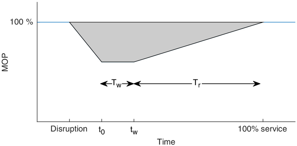
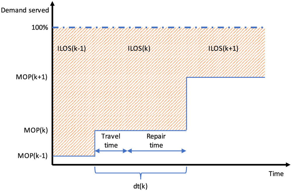
The effects of recovery on system performance are quantified by the evolution of the measure of performance (MOP) upon disruptions and the associated resilience phases as shown in Fig. 1. The MOP at time is expressed as the percentage demand served at time . The difference between the 100% MOP and the current MOP value is the demand not served at any time; integrating the demand not served through the recovery yields the cumulative demand not served, referred to as the integral loss of service (ILOS) (gray shaded area in Fig. 1). After a disruption, the absorption capability lessens the impact to the MOP. Recovery starts at time , the effect on the MOP is seen after the completion of the first repair, at and spans over the time .
Grid operating organizations commonly face two challenges related to power grid failures. First, in the planning stage the challenge is to design more reliable networks and response plans, addressing the absorption capability through grid hardening (National Academies of Sciences and Medicine 2017). The second challenge is managing the repair and restoration process in the operational stage, addressing the recovery capability, which aims at minimizing the demand not served and recovering as fast as possible, regardless of the initial postdisruption state of the grid (Arab et al. 2016). Thus, efficient implementation of grid recovery, based on thoroughly assessed plans, critically contributes to power grid resilience (National Academies of Sciences and Medicine 2017).
Damage assessment is the first recovery step in the case of large-scale damage to the grid (Çağnan et al. 2006), providing repair time estimates and thus the basis for repair planning. Damage assessment typically consists of an aerial survey, which identifies malfunctioning lines and delivers a coarse estimate of repair times based on the detected damage severity. The following ground survey carried out by linemen inspection crews refines these estimates (T&D World 2016). The complete assessment usually spans from (Nowak 2018).
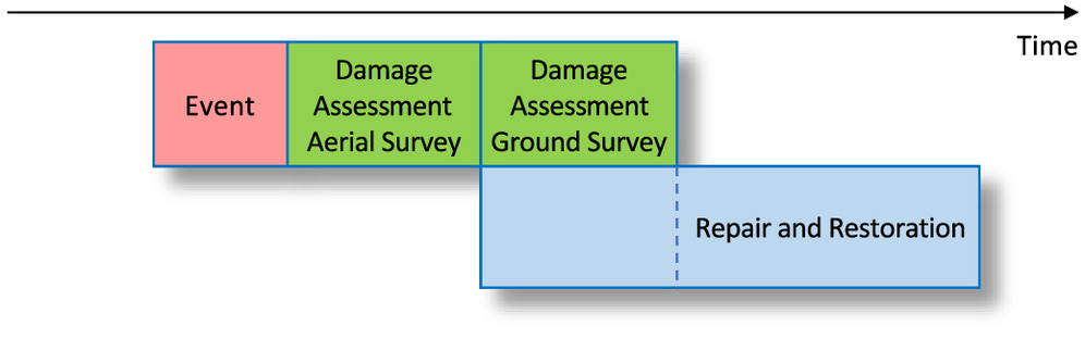
In practice, repair planning and repair, i.e., crew deployment and routing over the road network, are not initiated until damage assessment is complete. Furthermore, damage information is increasingly available in real time due to the digitalization of the damage assessment process (Nowak 2018). Consequently, planning and repairs can be initiated earlier, which could speed up the overall service restoration. However, this implies planning on the basis of preliminary damage assessment results and the capacity to replan as the damage estimates are refined. This paper examines the potential of the receding horizon planning approaches and specifically evaluates the model predictive control (MPC) method for this application. These approaches incorporate updated damage estimates on a rolling basis in a continuous replanning process. The process sequence of this approach is shown in Fig. 2. Subsequent to the event, damage assessment is carried out followed by repair and restoration. The overlapping part shows the gain from initiating the repair and restoration process sooner before waiting for the completion of the ground survey. The conventional approach of waiting until the complete damage assessment information is available before preparing a definitive repair plan is seen to correspond to an open loop approach.
Therefore, the contribution of this work is to minimize the ILOS of a damaged transmission grid by starting the repair process early even with limited damage information to reduce the waiting gap (in Fig. 1, the difference between and includes both the waiting gap and the time to complete the first repair). Second, by updating the repair planning continuously with the most recent damage information to enable replanning of the scheduled repair actions and grid operations.
Based on receding horizon model predictive control (MPC), which allows dynamic replanning based on damage information updates, this work addresses three questions:
1.
Does the MPC approach improve the repair performance compared with the current industry standards?
2.
Which factors affect the MPC performance?
3.
What is the minimum MPC planning horizon that yields an acceptable level of performance?
The remainder of this paper is organized in sections as follows. The next section examines the literature and research gaps leading to this work. The section “MPC Approach for Repair Planning of Power Grids” discusses the methodology of damage assessment and repair planning under the open loop (OL) and MPC approach, the modeling of the power grid, road network, and repair planning. The section “Case Study” introduces the IEEE39 bus network to answer the three aforementioned research questions. Thereafter, results and discussion and findings are presented. The paper is concluded with final observations and suggestions for future work.
Relevant Literature
Previous work on power grid recovery following disruptions addresses the construction or assessment of recovery strategies and plans. The former includes handling of multiple teams and the economic minimization of repair costs. Assessment studies, on the other hand, cover analyses of existing recovery strategies, policies, and plans through simulation or comparative analysis.
Assessments have especially focused on preformulated strategies (PJM Interconnection 2017) which are used in the power transmission and distribution industry for the ordering of repair actions. In Çağnan et al. (2004, 2006), discrete event simulation is used to examine how access times, repair times, spare part delivery times, and the stocks of spare parts affect the performance of repair strategies and plans. The stochastic simulations show that the difference between actual repair times and logistics and their preplanned values might affect the order of the whole plan and the total repair time. The authors conclude that there is a potential for the optimization of repair planning and logistics.
For the construction of repair plans subject to a specific damage, Van Hentenryck et al. (2011), Coffrin et al. (2012b), Coffrin and Van Hentenryck (2015), and Van Hentenryck and Coffrin (2015) show that an optimized repair order minimizing the demand not served, accelerates the repair process and minimizes the economic impact of outages in damaged transmission grids. The associated mixed integer problem with a nonlinear objective function and linear constraints is solved by decoupling the problems of repair order and the optimal repair crew routing (Van Hentenryck and Coffrin 2015). The use of the repair order as precedence constraints in the scheduling problem is known as constraint injection, and it is used to schedule multiple teams through a vehicle routing problem. However, this does not necessarily result in global optimal solutions, which minimize the blackout size over time raising the question. Assuming perfect damage, repair time, and access time information as done in (Van Hentenryck et al. 2011; Coffrin et al. 2012b; Coffrin and Van Hentenryck 2015; Van Hentenryck and Coffrin 2015) makes replanning unnecessary, but is unrealistic.
Tan et al. (2019) present a multiteam scheduling approach for the repair and restoration optimization of distribution networks with radial architecture. To accommodate multiple crews, the authors introduce scheduling polyhedra within the repair order problem, which allows the whole problem to be solved within one stated optimization problem. The set of power flow is approximated as one-directional flows in the radial grid topology, simplifying the AC power flow equations significantly. However, as shown by Coffrin and Van Hentenryck (2015), reactive power flows are required to describe a transmission grid during restoration and repair. Furthermore, only repair times are considered but not traveling times between the sites. Tan et al. (2019) assume perfect damage and repair time information and discuss the possibility of replanning the repair order due to updated damage information (Tan et al. 2017).
Morshedlou et al. (2019) extend the problem of repair planning to general complex infrastructure networks with an application of the DC power flow model to the French system. Contrary to the other models discussed, the allocation of multiple repair crews for one line and the partial operability of damaged components are being considered. Further, complete damage information is being assumed, but the possibility of real time execution is mentioned but not further investigated.
Xu et al. (2019) compare methodologies for solving the repair planning problem in terms of ILOS performance given damage scenarios caused by various seismic intensities. These include component importance-based methods, genetic algorithm-based methods, and time index-based heuristic and component index-based exact solution methods. A combination of the index-based heuristic method and the component index-based exact solution method is shown to achieve the best ILOS performance. However, the model does not consider changing damage assessment information or updating and replanning.
A different approach on optimization is taken by Arab et al. (2016). Contrary to the other work presented and to our work, the authors aim to minimize the economic costs of disruptions, considering for disaster economics such as hourly crew costs, generation costs, shutdown and startup costs. However, this approach assumes constant economic value of transmission lines and simple linear flows on the transmission lines. As shown by Coffrin and Van Hentenryck (2015), however, this does not reflect the realistic power flows of grids during restoration. Nevertheless, this assumption allows for modeling the problem as a linear program with an exact solution through Benders decomposition. Updating or replanning are not considered in this contribution, because repair costs are considered as fixed given parameters.
The aforementioned studies do not consider the damage assessment as an ongoing process, providing accessible but changing repair time estimates. In turn, the resulting waiting gap that causes additional ILOS is not taken into account, because these studies assume that repair planning begins with perfectly accurate repair time estimates once the damage assessment is fully available. To overcome the waiting gap limitation and to utilize real time information, Van Hentenryck et al. (2012) employed the online stochastic combinatorial optimization (OSCO) methodology to solve the problem based on fragility modeling. The authors suggest that a mixed approach of OSCO and conventional damage assessment shows the best performance. However, one essential assumption is that damage assessment teams conduct repair, which is not in agreement with the industry standards, as presented in (T&D World 2016; Nowak 2018; Çagnan et al. 2004). To our knowledge, this is the only work which considers actual repair times that may differ from predicted repair times; however, this work does not derive the repair times from a damage assessment based on aerial survey and ground survey but from simulation.
A widely used approach to face real time information in multistage optimization problems is model predictive control (MPC) (Camacho and Alba 2013), which has shown to be suitable for dynamic decision-making problems requiring replanning (Sethi and Sorger 1991). The receding horizon approach, as a central idea of the MPC, solves the control problem for the next steps, only applies the first step of the solution and, then, repeats (Camacho and Alba 2013). The approach is advantageous if the full horizon is not solvable, or for reducing the computational burden. MPC has been successfully applied for operational restoration planning including black-start and re-energization, incorporating real time information and system state feedback (Qiu and Li 2017; Golshani et al. 2017; Gholami and Aminifar 2017). For combinatorial problems, such as vehicle routing problems and traveling salesmen problems, which are relevant to the repair planning as used in (Van Hentenryck et al. 2011; Coffrin et al. 2012b; Coffrin and Van Hentenryck 2015), receding horizon approach has been studied in the operations research, game theory, and decision-making context (Sethi and Sorger 1991; Kimms and Kozeletskyi 2016; Perez et al. 2013).
In summary, the optimization-based planning of repair order and repair crew routing has been addressed in the literature. However, existing approaches assume perfect information on damage extent and repair times. This work examines the implementation of the MPC concept to address one of the gaps in the repair planning, i.e., the evolving state of information and the consequent replanning and aims to evaluate its feasibility and performance.
MPC Approach for Repair Planning of Power Grids
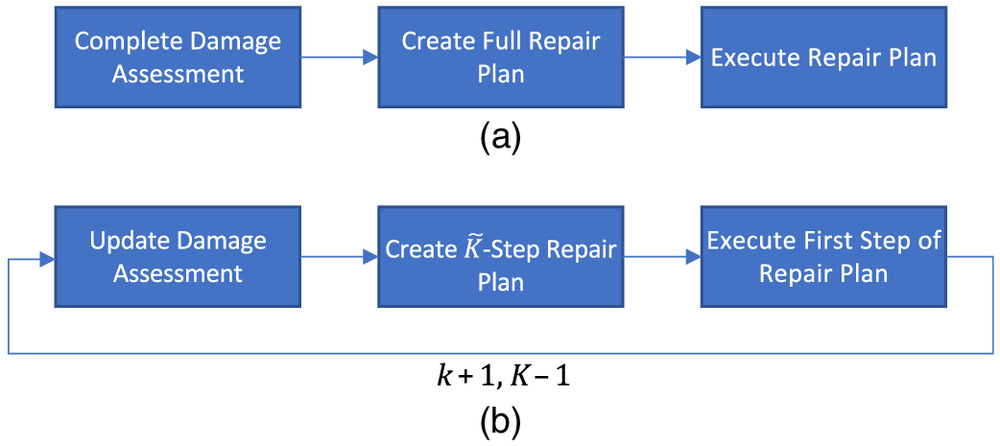
To quantify the potential of the MPC approach, its performance is compared in this section with the Open Loop baseline approach. The latter follows the common repair planning strategies presented in the literature (Van Hentenryck and Coffrin 2015; Tan et al. 2019; Xu et al. 2019) and entails a sequential damage assessment, repair planning, and repair execution process for all damaged lines as shown in Fig. 3(a).
Once the damage assessment is completed, the repair plan is created for a whole set of damaged transmission lines and executed subsequently. Given the availability of exhaustive damage assessment and precise repair times, the solution to the repair plan problem produces the optimal repair sequence. However, this comes at the cost of waiting until the ground survey is completed and hence of increased ILOS.
MPC Approach
To overcome the limitation of waiting until the complete damage assessment information is available, the MPC approach can formulate the repair plan and execute it as soon as the first piece of information is available, i.e., the ground survey of the first inspected transmission line in this model as shown in Fig. 2. Embracing the MPC vocabulary, the repair planning for the damaged lines is executed in a receding horizon scheme with the planning horizon based on a mix of aerial survey data and data from the ongoing ground survey. After the repair of the next transmission line, which marks one step of the current plan, the repair planning problem for the remaining damaged lines is solved again by incorporating the updated ground survey information as shown in Fig. 3(b), which marks one iteration of the repair planning process. After a line is repaired, it is removed from the set of damaged lines, and the location of the latest completed repair is used as the updated starting location for the routing of the repair crew in the next planning iteration.
A similar concept of MPC which accounts for traveling to control the state evolution is Mobile MPC (MoMPC) which merges replanning combined with travel times and has been applied for the manual control of irrigation channels (Maestre et al. 2014).
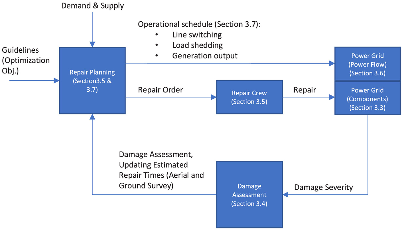
Fig. 4 shows the damage assessment and repair planning/execution scheme for the baseline and MPC approach. The damage assessment uses the result of the inspection by aerial survey and ground survey and produces repair time estimates, which are updated during the ongoing ground survey and are available in real time to the repair planning. The repair planning allocates the repair crews and determines the operational schedule by solving a joint optimization problem with the objective of minimizing the ILOS to fulfill the demand while utilizing the available power supply. The repair plan is executed by the routing of the repair crew, which performs the repair actions, and, concurrently, the operations, i.e., line switching, load shedding, and generation output control are jointly coordinated by the TSO, who leads the repair and operations planning.
The power grid is represented by two system perspectives, i.e., by the grid transmission assets and by the corresponding operational features described by the power flow equations. The OL and the MPC approaches are executed according to Figs. 3(a and b), respectively. In particular, the OL approach executes the planning only once after the completed damage assessment; conversely, the MPC approach runs a new iteration of repair planning after a repair of a transmission line has been accomplished based on the most recent update from the damage assessment.
The developed MPC approach for the repair planning of power grids is framed as an optimization problem with the objective to minimize the ILOS. Its key components are introduced in the remainder of this section. The next subsection describes the resilience metrics and objective function of the optimization problem. The structure and operations of the power grid and road network, the damage assessment and the repair processes are represented as constraints in the optimization problem. In particular, the following subsection introduces the spatial model of the grid and of the road network, which is used for the damage assessment and the repair planning presented thereafter. After the description of the power grid operational model, finally, the section is concluded with a presentation of the overall optimization problem combining the aforementioned objective and constraints.
Resilience Metrics and Optimization Objective
The increase of the recovery capability of the power grid, focusing on the ILOS for the affected customers, is achieved in three stages, namely: (1) by shortening the time , which is the timespan between the start of damage assessment and the completion of the first repair action, as shown in Fig. 1; (2) by the repair order optimization during the timespan ; and (3) by the optimal scheduling of loads and power injections at each repair stage computed by optimal power flow operations.
Given the active power being served to the load at bus , the MOP is defined by the demand served over the whole grid:
(1)
These power injections are determined by the demand, supply, and the power flow depending on the current grid topology available. Conversely, the loss of service (LOS) is defined by the difference of the nominal total demand and the MOP, i.e., .
To measure the overall performance of the recovery phase, the ILOS quantifies the energy which has not been served to all customers in the grid over the recovery and is defined by the integral of the loss of service over time. Given the discrete steps defined by the repair actions of damaged lines, the ILOS is calculated as:
(2)
This is illustrated in Fig. 5 for one time step . The time difference between two consecutive repair actions consists of repair time and travel time. Indeed, travel times can have a non-negligible impact on the ILOS especially in case of limited repair crew resources. Thus, the ILOS depends on initial LOS, the LOS levels following the power grid repair actions by the operations, i.e., the solution of an optimal power flow, given the current grid topology and the time in between those repair actions.
Spatial Grid and Road Network Representation
The power grid consists of geographically distributed components, i.e., substations (buses) and transmission lines made up of diverse components, namely, line segments, towers, and poles. Transformers are located at the substations and are modeled as part of a transmission line with negligible length. Damage assessment and repair crews can access substations through the road network. To reduce the problem complexity caused by the large number of locations requiring inspection and repair, transmission lines are modeled as starting and ending at substations. The geographical properties of a transmission line are characterized by its start and end locations. The length is the Euclidian distance between those buses. Every component of a transmission line can be accessed through a service road or off-road terrain from the start or the end point of a transmission line. To enable the crew routing, the matrix is constructed from the road network with each entry describing the shortest path travel time between substations and .
Damage Assessment
The estimated total repair time of a transmission line is quantified based on its damaged components and their damage severity. Because no repair planning data are available prior to the aerial survey, the aerial survey must be completed before any planning is performed (in the baseline and in the MPC case). The time marks the end of the aerial survey and the beginning of the ground survey. Therefore, the aerial survey contributes to the waiting gap (as presented in Fig. 1) in the same extent in the baseline and in MPC cases.
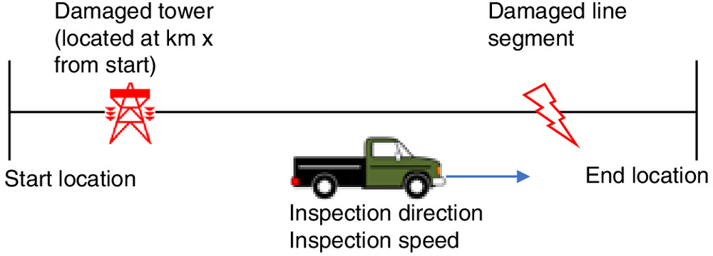
The ground survey is carried out by inspection crews, traveling along the damaged transmission lines with a given speed and recording the detailed damage of all components affected as defined in the Appendix. Contrary to the aerial survey which can only estimate the damage extent of a line, the ground survey inspection crews provide detailed assessments on site. This provides an update to the estimate of the damage severity from the aerial survey and, thus, of the total repair time of the transmission line. Because in practice, the ground survey identifies the parts needed for repairs; hence, repair crews cannot start repairing a transmission line until the ground survey is completed.
Fig. 6 illustrates the ground survey process for one transmission line with two damaged components. Updates to the ground survey are reported immediately and become available to the repair planning process; therefore, repair time estimates rely on aerial survey data, ground survey data or a mix of both if the ground survey on the particular line is still ongoing. Thus, the most recent repair time estimate for of transmission line is computed as:where = set of components where only the aerial survey is available, whereas represents the set of components for which the ground survey has been completed with corresponding repair time estimates and . The derivation of these estimates is presented in the Appendix under “Damage Severity” based on the component type and damage level classification. The conditional probabilities that the aerial survey correctly classifies the damage level are listed in the Appendix under “Damage Assessment.”
(3)
The ground survey needs to be scheduled optimally to minimize duration and to ensure that lines with the highest impact to the service restoration are released for repair first and repair allocation to subordinate transmission lines is subsequent. This is achieved in two stages, i.e., (1) a preliminary repair order is calculated without considering travel and repair times as in Van Hentenryck and Coffrin (2015), and (2) the sequence obtained is used as an importance ranking for scheduling the ground survey inspection crews, the extremity of transmission lines at which inspection begins, and the routing. The schedule is obtained through a round-robin scheme (Rasmussen and Trick 2008), i.e., the lines to be inspected are allocated to inspection crews in order of descending importance.
Considering the inspection order, the travel times over the road network and the total ground survey inspection time of a line , its ground survey finishing time can be calculated. The minimum ground survey finishing time determines the earliest start of the repair process.
Cooptimization of Repair Planning and Operations
Based on the damage assessment, demand and supply and service guidelines, two intertwined plans are developed through one joint cooptimization approach that minimizes the ILOS. These are the repair plan, identifying the sequence of repair actions and locations, and the operations plan, identifying when to activate repaired transmission lines and how to dispatch power generators and perform load shedding subject to the available topology and power flow limits.
Repair Planning
Repair planning is characterized by the following features:
1.
The main repair planning guideline is to minimize the total demand not served, i.e., the ILOS. The guideline is general and can be tailored to specific preferences of the system operators;
2.
In the repair order problem, the damaged components are characterized by the repair time calculated from damage severity;
3.
Logistic issues, i.e., material and replacement components, are not explicitly considered;
4.
The repair of a transmission line starts at either endpoints and ends at the opposite side;
5.
The travel speed of repair crews is on roads and along the transmission lines between the repair actions; and
6.
The repair of a damaged line can only start if the corresponding ground survey has been completed to ensure that spare parts will be on site.
Each line can be accessed by the two buses it connects; therefore, travel combinations exist between lines and . Hence, for every additional damaged line to set , travel combinations are added and thus, the set has a total of travel combinations. The crew routing is described by the variable , which takes the value 1 if the crew travels from bus of line to bus of line , performs the repair of line and completes the task at bus during step . Thus, the time estimate associated with this repair schedule is:where = shortest path travel time between bus and , and = repair time estimate of line . Accordingly, and are vectors of the values of and .
(4)
To complete the repair, all damaged transmission lines must be visited. The following constraint prevents that a line gets visited twice in opposite directions:
(5)
Eq. (5) is formulated as an inequality to accommodate for the planning horizon and is an equality in the OL case. Here, we assume one repair crew which can travel one path at a time. Thus,holds for all permutations of , . Furthermore, a crew can only depart from and arrive to a line, which is formulated by the constraint:
(6)
(7)
The time difference between the steps and is represented by as illustrated in Fig. 5. To exclude the case that no damaged transmission lines are available for repair because the damage assessment is still ongoing, the waiting time is introduced. With the constraint, Eq. (6) which allows only one entry of to be 1, the time difference can be calculated by:
(8)
The MPC receding horizon scheme and the quantification of the performance of a repair plan require that the scheduling and completion of repair actions be related to a common reference time. To this aim, the total elapsed time at step is introduced:
(9)
is initially set as the completion of the aerial survey time. In the receding horizon, needs to be set for every new planning iteration to of the previous planning iteration to keep account of the elapsed time. Due to the logistics issue of spare parts, the repair of a transmission line cannot start before its ground survey completion time . This is enforced by the constraint:
(10)
To indicate that a line has already been repaired at time step , the indicator variable , , is introduced as:and . For the repair planning of the MPC approach, the transmission lines already repaired are removed from the set of the damaged lines , which is updated at each planning iteration. The repaired lines are not included in the remaining planning.
(11)
Power Grid Model
In the power grid, any bus can host loads and generators, and is characterized by the active power injection and reactive power injection . The active power flow from or into the bus , is calculated by:where = active power flow on the transmission line connecting buses and . For the reactive power flow, . If , then the bus represents a net generator bus. The net power injections by generators and the withdrawal by loads of active and of reactive power at bus are characterized, respectively, by the lower bounds P_i and Q_i and by upper bounds P_i and Q_i. Further, the electric properties of a bus are described by its bus bar voltage and phase angle. The transmission lines are described by their conductance, susceptance, and thermal line flow limit .
(12)
Because the grid is in the recovery state and not at its normal point of operation, the DC power flow approximation does not match the AC solution sufficiently as it neglects reactive power flow and bus bar voltages (Coffrin and Van Hentenryck 2015). Therefore, the AC power flow equations are approximated by a linear programming approach which is known as linear programming AC (LPAC) (Coffrin and Van Hentenryck 2014). This approach approximates the cosine function of the phase angle difference in the power flow equations as LPAC with the selection of the best linear functions as approximations by solving a linear optimization problem.
To schedule grid operations, two sets of decision variables are considered, i.e., (1) which lines are in operation, and (2) how to shed load and how to set the generator feed-in. The former set accounts for the Braess’s paradox, i.e., a repaired line should be kept out of operation if this leads to a larger power supply. This is implemented by introducing the variable indicating if the line is operational with the constraints
(13)
(14)
The second set of variables constrains the power injections and to minimize the ILOS and ensure safe operations. Therefore, transmission lines can only transmit power when in operation and must not be overloaded, i.e., the apparent power must stay within its thermal limit :
(15)
Cooptimization Formulation
After introducing the objective function, damage assessment, repair planning and power flow, the whole optimization problem is formulated as the following mixed integer problem:
(16)
The objective function in Eq. (2) and the constraints presented in the section “MPC Approach for Repair Planning of Power Grids” result in mixed integer nonlinear programming. As the cosine functions of the power flow equations are linearized by the LPAC approximation and the apparent power limitation constrains are replaced by a piece-wise linear approximation as explained in the subsection “Power Grid Model,” only the objective function term minimizing the ILOS remains nonlinear. This allows precomputing the power flows according to every possible repair action over the steps as linear optimization problems. Eventually, the best sequence can be obtained by assessing the objective function terms which minimize the ILOS.
Case Study
To assess the viability of the MPC approach, its performance is contrasted against the performance of the baseline approach for the same scenarios. To answer the question, “Which parameters impact the MPC performance?” we focus on those parameters that have an immediate effect on the uncertainty of the repair time estimates following the aerial survey, because the MPC approach particularly relies on them for the initial planning. As the most crucial parameters, we identify the quality of the aerial survey and the damage severity given by the number and damage level of components affected per line.
Whereas the damage severity and aerial survey quality address situation- and scenario-specific parameters, we additionally assess the main algorithmic parameter, i.e., the prediction horizon of the MPC approach defined as the number of repair steps ahead calculated in the receding horizon. Our analysis starts at one step prediction horizon up to five steps, determined by the limits of the available computational power.
Demonstration System
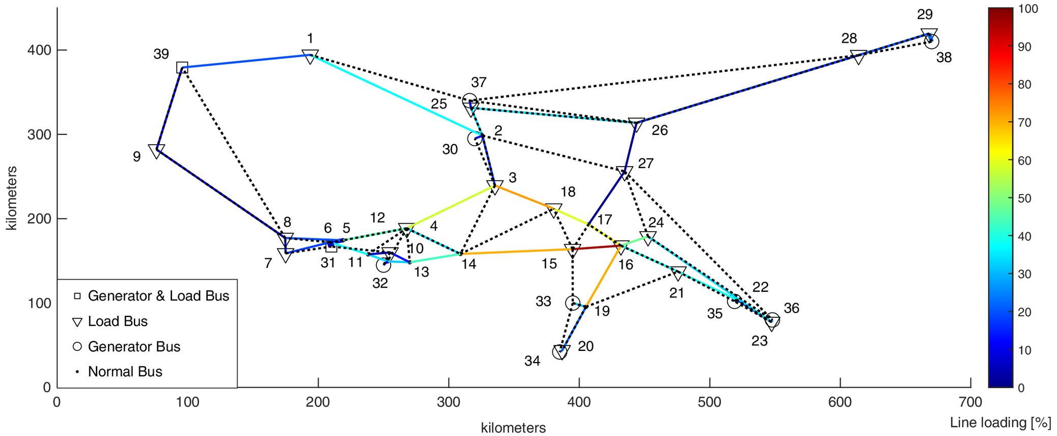
The IEEE 39 bus system (Carr 2013) is used for demonstration purposes. It resembles the size of a regional transmission grid consisting of 39 buses with 10 generators, 19 loads, and 46 transmission lines. Published spatial data are only available for a part of the grid (Manitoba Hydro International 2018). Subsequently, the spatial grid properties are calculated by multidimensional scaling from impedance-per-km industry standard values (Manitoba Hydro International 2018) and shown in Fig. 7. The line colors indicate the percentage of thermal loading limit in steady state operation. The artificial road network, represented by the dotted black lines, is based on Euclidian distances.
Simulation Parameters
Table 1 presents the simulation parameters whose impact on the MPC approach performance is assessed. Row one of Table 1 describes the value ranges over which the parameters are varied. The damage scenarios are characterized by the damage topology, i.e., the number and the spatial distribution of the affected lines, and by the damage severity, i.e., the number and type of damaged components and their damage levels per each affected line. The maximum of damaged lines is set as 15 which represents a severe contingency involving a third of all lines. The minimum is set to seven lines to be beyond the maximum prediction horizon, to avoid confounding the effect of the prediction horizon with the damage levels such that this effect can be quantified and analyzed. The quality of the aerial survey refers to the conditional probability of classifying the correct damage level and the resulting deviation between assessed and true component repair time based on the true damage level. Rows two to four of Table 1 describe the properties and implications of the parameters. The parameters with the property algorithmic have a direct impact on the problem size and on the solution approach, i.e., OL or MPC. Damage specific parameters cover the parameters defining the damage extent, i.e., the exact damage topology and severity. Damage assessment specific parameters cover the aerial survey quality. The parameters impacting the damage assessment quality have an impact on the discrepancy between estimated and real line repair times used in the repair planning. The effect of their variability is discussed under “Which Factors Impact MPC Performance?” Further details on the range of variability of the parameters are provided in the Appendix.
| Parameters | Repair planning approach | Prediction horizon | Aerial survey quality | Damage topology (number of damaged lines) | Maximum number of damaged components per line | Damage level of individual components |
|---|---|---|---|---|---|---|
| Parameter variations in simulation | ||||||
| MPC, open loop | One–five steps | Perfect, poor | 7, 12, 15 | Max 10, Max 50 | No damage, light damage, heavy damage | |
| Parameter properties/implications | ||||||
| Algorithmic | X | X | — | X | — | — |
| Damage specific | — | — | — | X | X | X |
| Damage assessment specific | — | — | X | — | — | — |
| Impacting the damage assessment quality | X | — | X | — | X | X |
Results and Discussion
Does the MPC Approach Improve the Repair Performance Compared with the Open Loop Approach?
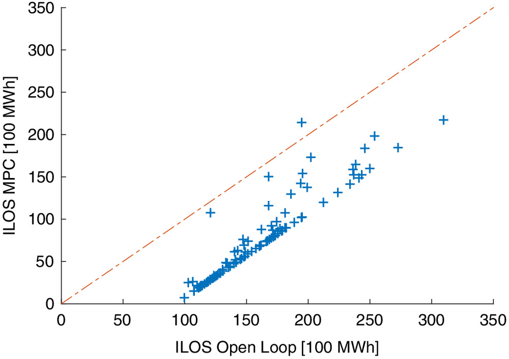
This section focuses on comparing the performance of the MPC approach relative to the OL approach, in terms of the resulting ILOS (lower is better). We show this by direct comparison between MPC and OL simulation results in scatter plots and by exceedance probability plots over all simulations; further, the maximum ILOS range of the two approaches is compared in percentage to each other. This is conducted in two stages: first, one topology, i.e., the set of affected lines, is fixed. This enables to show the performance increase in the scatter plot, given that the waiting gap is always the same. To vary the damage severity which has an impact about the repair order and aerial survey, 100 severities are generated, i.e., number of damaged components, their positions and damage levels and aerial survey results are generated for each of the seven lines. Because this work intends to show the broad applicability of the MPC methodology over any topology, in the next stage, 30 random damage topologies are generated. For each of these topologies, the algorithms are assessed for 20 different severities.
To show the benefits of starting the repair early even with limited information, relying partially on the aerial survey, Table 2 shows one damage topology with seven lines, and Fig. 8 shows the comparison between the OL and the MPC approach. Each datapoint shows one realization of severity. If a datapoint is below the dash-dotted line, the MPC approach outperforms the OL approach for that damage scenario, which is the case except for one out of the 100 scenarios. In the under-performing case, the first transmission line scheduled for repair in the first planning iteration is selected due to its large impact on the MOP and its short repair time. However, due to aerial survey quality, this repair time has been underestimated, whereas the repair times of other transmission lines associated with smaller MOP contributions have been overestimated. The combination of the aforementioned factors results in the underperformance of the MPC approach as compared with the OL approach.
| Line No. | From bus | To bus |
|---|---|---|
| 1 | 3 | 4 |
| 2 | 3 | 18 |
| 3 | 14 | 15 |
| 4 | 15 | 16 |
| 5 | 16 | 17 |
| 6 | 16 | 19 |
| 7 | 17 | 18 |
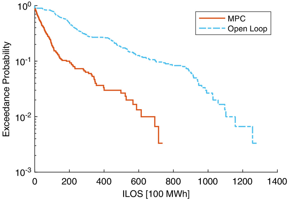
To quantify and compare the overall performance of the MPC approach, Fig. 9 shows the overall exceedance probability for 30 different damage topologies and 20 severities for each damage topology. The exceedance probabilities for the MPC curve is dominated by the OL curve and, therefore, the probability of exceedance for a given ILOS is smaller when applying the MPC approach for the repair. Furthermore, the maximum range of the OL ILOS is up to 73% larger than for MPC.
Which Factors Impact MPC Performance?
This section presents the case study results on the impact of the damage and damage assessment specific factors on MPC performance, again in terms of ILOS; the factors are the aerial survey quality, maximum number of damaged components per line, and damage level of components.
The simulations of the repair process use the parameter values as defined in the case study, and the damage topology is fixed to the same seven lines as defined in Table 2. The damage severity, which is quantified as light and high in the Appendix, is defined by the number of damaged components per line and the damage level per component. The probabilities of aerial survey damage classification are defined in the Appendix. The two scenarios of perfect and poor aerial survey represent the boundaries of the range of aerial survey accuracy. With these parameter variations, four different cases are simulated, namely, light severity and perfect aerial survey, light severity and poor aerial survey, high severity and perfect aerial survey, and high severity and poor aerial survey.
As shown in the previous section, the MPC benefits from starting the repair process before the completion of the ground survey. However, the MPC approach initially relies on repair time estimates from the aerial survey for planning the repair order, including uncertainty of repair time estimation. Hence, the main difference between the MPC approach and the OL approach is the starting time of repair and the ground survey information available to planning. Leveraging information update, replanning occurs in the MPC approach if the updated repair plan based on novel information improves the prospective ILOS.
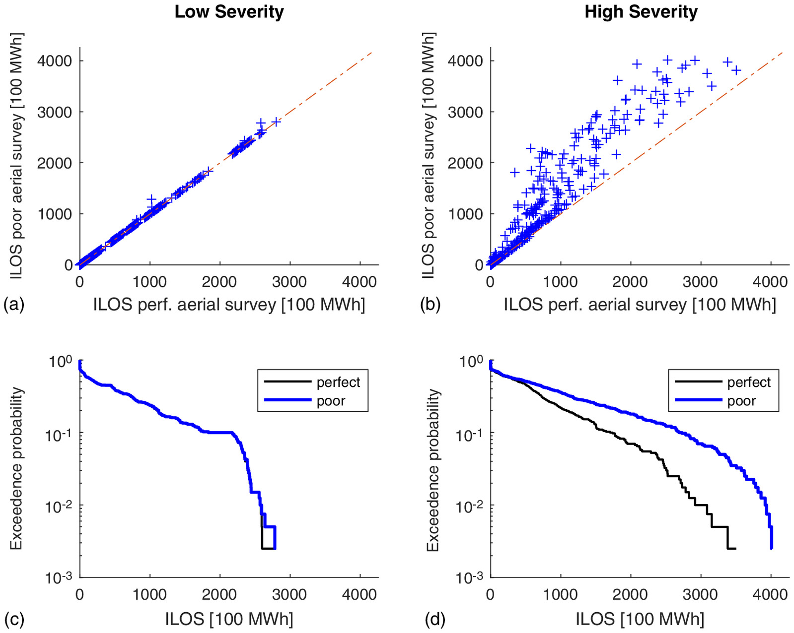
Eq. (3) states that the repair time estimation is the sum of component repair times and traveling time along the lines. Thus, the overall uncertainty is related to the variance of the estimated repair times. This variance of the estimation error for one single component depends on the accuracy of the aerial survey given the damage level. Further, the component damage level impacts the estimation error variance because the damage level classification outcome of the aerial survey is modeled by a conditional probability (see Appendix). The interplay of these factors is shown in Fig. 10. The left column of Fig. 10 illustrates the MPC performance given perfect and poor aerial survey under low damage severity. In the top-left scatter plot, the performance of perfect and poor aerial survey qualities within the MPC approach is demonstrated. As confirmed by the bottom-left exceedance plot, the difference in ILOS performance between the perfect and poor aerial survey scenario is not significant. However, in the right column, showing MPC performance under high damage severity, the MPC approach with poor aerial survey causes significant underperformance. This can be explained due to an increased variance of repair time estimates with an increasing number of damaged components.
With independent distributed estimation errors, two conclusions can be derived from Eq. (3) which explain the results in Fig. 10: (1) the higher the variance of the individual component repair time estimates, the higher the uncertainty; and (2) the higher the number of components per line affected by an estimation error, the higher the uncertainty of the overall repair time estimate because the variance of the overall estimation error increases.
Impact of the Aerial Survey Quality on Repair Time Estimation Uncertainty
The poorer the quality of the aerial survey, the more likely the estimated repair time deviates from the real repair time and deteriorates the prediction of the prospective ILOS. In this case, the replanning likely results in an improved repair sequence. If the aerial survey estimates of the damage severity are exact, the MPC approach obtains the same repair sequence as the OL approach. The difference in ILOS is determined, hereby, by the waiting time until the ground survey has been completed and the initial MOP resulting from the damage induced topology. Moreover, the modification of the repair sequence might lead to an increase of the travel time and, thus, accrue the ILOS as compared with the theoretical optimal order achieved by the OL approach. This happens if the travel time is comparable to the repair time, if the damage is widespread or if the number of crews is limited.
Fig. 10 illustrates the ILOS (upper row) and exceedance probability (EP) (lower row) for two different severity levels and quality aerial surveys of two equally damaged topologies. As expected, in both cases the perfect aerial survey yields the best performance. In the case of the high severity damage, the difference between the EPs for a given ILOS value increases, and a poor aerial survey causes a maximum range of ILOS which is 15% larger as compared with the perfect aerial survey.
If the travel time increases by due to the replanned sequence, this also increases the prospective ILOS by the cost of replanning:
(17)
Impact of Damage Severity on Repair Time Estimation Uncertainty
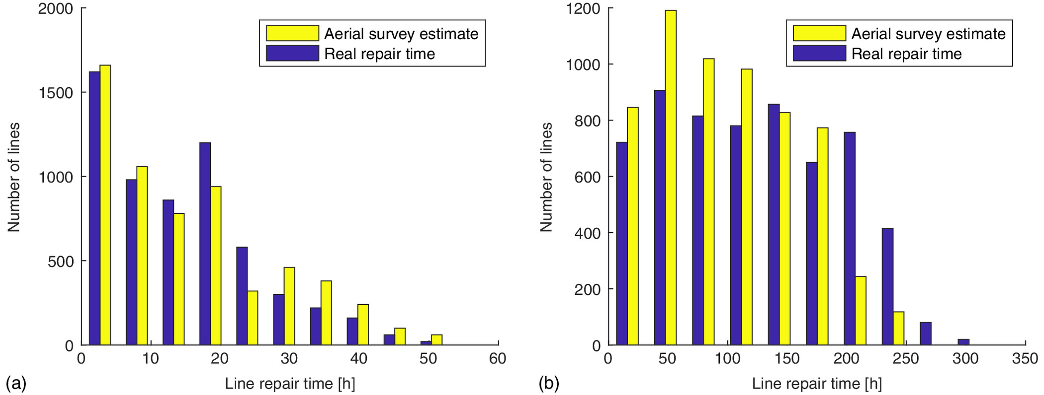
The increase of the number of damaged components increases the variance of the repair time estimates and, thus, the likelihood of suboptimal replanning. This is due to the cumulative effects of uncertainties in the components’ damage levels identified by the imperfect aerial survey. Moreover, the damage level of a component also influences the quality of the repair time estimates based on the aerial survey. Therefore, there may be a misclassification of the damage severity and the associated repair times as detailed in the Appendix under “Damage Assessment.” Fig. 11 shows the distribution of the actual and of the estimated repair times per line resulting from a poor aerial survey for 6,000 transmission lines. Fig. 11(a) shows the histogram for the case of light damage severity and Fig. 11(b) for high damage severity. A low severity with a maximum of 10 components per line with no damage or light component damage leads to a similar performance of the algorithm given perfect or poor aerial survey quality. This does not hold true anymore for a high severity with up to 50 components per line of light and heavy component damage level. For the light severity, the histogram shows less discrepancy between aerial survey and real repair times as for the high severity.
Is It Possible to Reduce the Planning Horizon of the MPC Approach?
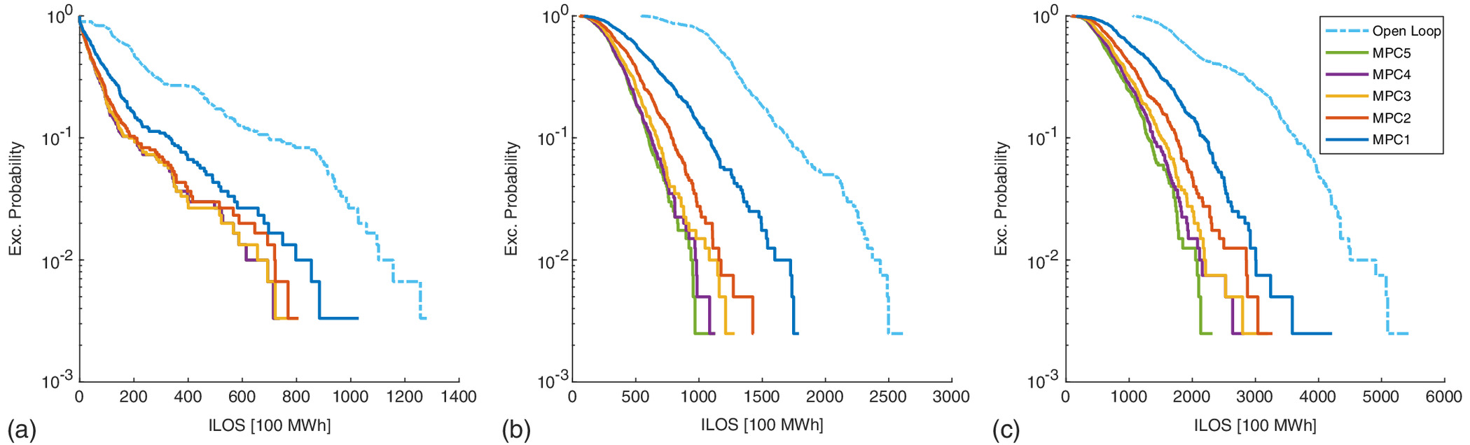
To the best of our knowledge, no clear algorithmic solution currently exists for the problem stated in Eq. (16). damaged transmission lines, which can be accessed from two sides, result in repair planning combinations using a prediction horizon of steps. This configures a combinatorial exponential growing state tree already at small problem sizes, if the full horizon is solved, and prevents application of the developed methodology to systems of realistic size. Therefore, this section investigates how the horizon length impacts the performance of the MPC approach. The ILOS performance associated with a certain horizon length of the algorithm might depend on a specific topology; therefore, 20 randomly sampled topologies are investigated with 20 different severities each. These problems are solved with MPC horizons ranging from one to five steps and with the OL approach to compare the performance in terms of ILOS. The EP plots for seven, 12, and 15 lines are shown in Figs. 12(a–c), respectively. It is clearly visible that all MPC approaches overperform the OL approach. The average performance increase of MPC with a prediction horizon of five steps versus OL is 78% for seven lines, 71% for 12 lines, and 68% for 15 lines. If the prediction horizon is reduced to three steps, these average performance increases decrease slightly to 64%, 68%, and 78%, respectively. The maximum ranges of the MPC approach with a prediction horizon of five steps versus the OL are 42% less for seven lines, 57% less for 12, and 15 lines. For a prediction horizon of three steps, these ranges are 37% less for seven lines, 51% less for 12 lines, and 41% less for 15 lines.
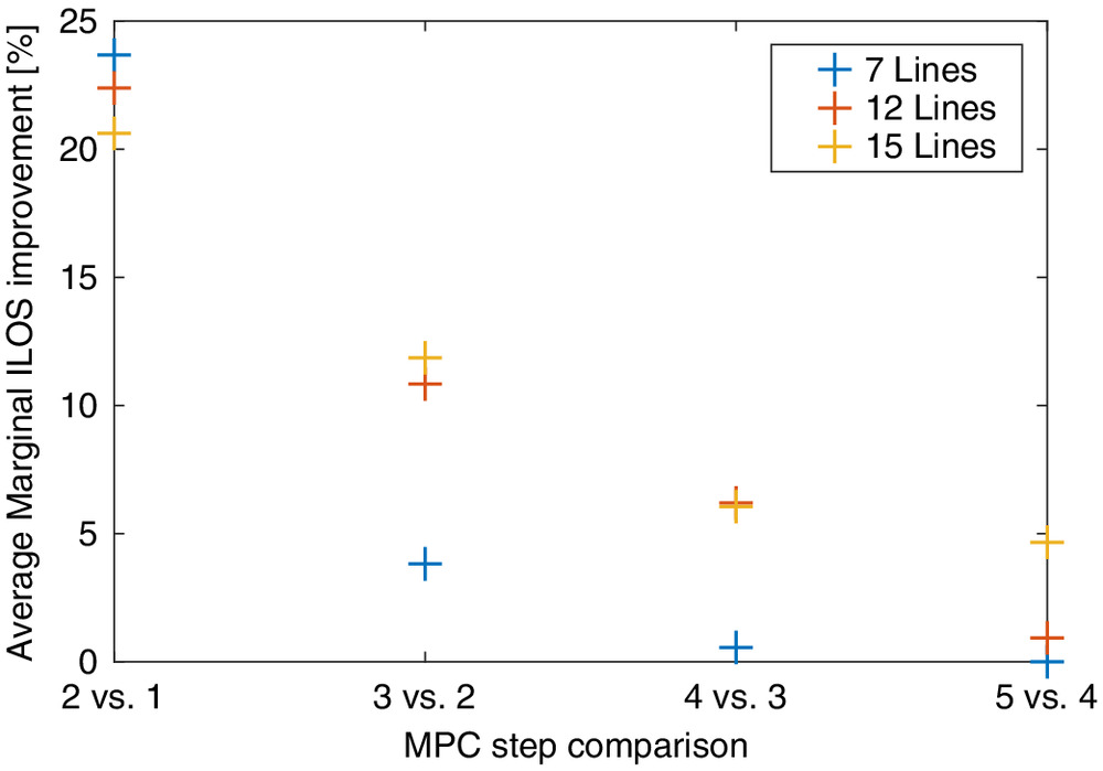
To further quantify the advantages of the MPC approach on a case-by-case basis, we compare the marginal ILOS improvement, , between two horizon lengths and . For the simulation , this is computed as
(18)
Respectively, we define the average marginal ILOS improvement, , between two horizon lengths and over all simulations as
(19)
Fig. 13 shows the average marginal ILOS improvements, , over all 400 simulations for 7, 12, and 15 damaged lines in the IEEE 39 bus system with MPC horizon lengths of one to five steps. For all cases as shown in Fig. 13, this average marginal ILOS improvement falls below 5% as the MPC prediction horizon exceeds four steps. A further observation is that at a given MPC planning horizon , is higher for the case of a higher amount of damaged lines. This allows the interpretation that damaged topologies with a higher number of damaged lines require a higher MPC prediction horizon.
Benefits of the MPC Approach to the Repair Planning
Waiting Gap and Replanning
If the quality of an aerial survey is perfect, the MPC approach has access to the correct planning data from the beginning which results in the same repair sequence as the OL approach. By definition, the OL approach starts the repair work not before the last line’s ground survey has been finished, whereas the MPC approach is capable of starting the first repair work by the time the first line’s ground survey has been finished. The time difference of these two different starting times is the waiting gap which is the time advantage of the MPC approach. Given the initial MOP after the damage with , the integral loss of service waiting gap () quantifies the advantage upper bound of the MPC approach and is calculated by
(20)
Given that the OL approach is provided with the full ground survey information, it is possible to compute the optimal repair sequence. The MPC approach, however, relies on a mix of aerial survey and already completed ground survey data. Hence, only in a best-case scenario the MPC approach finds the same sequence with an ILOS of . This sets the as an upper boundary of over-performance against the OL approach.
Replanning based on updated information might improve a suboptimal trajectory during the overlap of ground survey and repair. Because the ILOS is composed of time and LOS, additional travel time results in a higher additional ILOS in the beginning when the MOP is particularly low. Thus, if many repair actions are scheduled during the overlap, it is more likely for them to be rescheduled. Furthermore, the more information and completed ground survey results are obtained within the overlap, the more likely is the case of replanning. Given these considerations, the MPC can especially play its advantage in the case of large-scale damage in topology and severity causing ground surveys of long duration. If the overlap is long, the waiting gap will increase, and thus the benefit of starting early increases. However, after the whole ground survey has been completed, no replanning will happen anymore because information will not change.
Future Trends of Damage Assessment and Repair Planning
Especially the first repair actions are depending on the ground survey scheduling because repair can only start on those lines which damage assessment has been completed. Thus, the ground survey and its scheduling are critical for both the OL and the MPC approach. Whereas for the OL approach only the duration of the whole damage assessment is of interest because it determines the waiting gap; it has a direct impact on the repair sequences being determined in the MPC approach. As explained in the subsection “Waiting Gap and Replanning,” the durations of repair actions in the beginning have a higher impact on the resulting ILOS than the repair actions in the end when the MOP is already close to 100%. If the quality of the aerial survey is increased, the MPC approach will be less prone to suboptimal planning due to deviating information. On the other hand, if the duration of the ground survey gets shortened, the ILOS of OL approach and the MPC approach will converge because the advantage of starting early vanishes, and information will be fully available after the short ground survey. This last point leads to the future perspective of the damage assessment process. As recently reported (Pasztor 2017), drone inspection will be used in the future for the damage assessment as it has been successfully tested. Depending on the number of drones available and due to their speed compared with ground survey crews, this might blur the line between aerial and ground survey which might be combined eventually. Due to a smaller distance to the damaged components, the damage classification is likely to be more precise. This will allow to decrease the waiting gap to a minimum and improve the repair planning data quality.
Conclusion and Future Work
The benefits from starting the repair process for the power grid while the damage assessment is still ongoing was presented in this work.
The most significant benefit is drawn from starting early, whereas replanning supports especially the correction of suboptimal repair sequences. In our simulations, we have shown that this results in an average ILOS performance increase of up to 78%. However, we highlight that the performance increase of the MPC approach decreases in the case of replanning where travel-intense correction becomes necessary. A notable derivation we have made is that the performance increase is bounded by the waiting gap determined by ILOS due to waiting for complete damage information. Further, we have demonstrated in our simulations that every factor, increasing the variance of the repair time estimations, i.e., number of damaged components and aerial survey estimation variance, increases the probability that an ongoing sequence is suboptimal and might need to be replanned at the cost of additional ILOS.
The main limitation of all approaches presented are that the solution at every receding horizon step is performed brute force with an increasing number of operations necessary with increasing number of damaged lines or increasing number of prediction horizon steps. Furthermore, our investigations were limited to one repair team in this work. Thus, for further work, the MPC approach has to be extended to accommodate multiple repair team planning. The solutions of Van Hentenryck and Coffrin (2015), Arab et al. (2016), and Xu et al. (2019) have not been compared yet in terms of quality to our brute force MPC approach. For MPC for a smaller number of teams, a sensitivity analysis needs to be carried out on how the solutions of those approaches are converging with an increasing number of teams. As one option to extend our approach for multiple teams while incorporating the asymmetric feature of the traveling times which are of significance for a certain level of damage severities. Additionally, as mentioned in the subsection “Future Trends of Damage Assessment and Repair Planning,” the cooptimization of the damage assessment needs to be further emphasized in future work because it has a significant influence of the solution quality.
To demonstrate the applicability to real world problems, further work should cover case studies of existing power grids and road networks. Realistic damage topologies might be sampled from, e.g., earthquake probability distributions for the given area. This might open up a further potential of case studies, revisiting existing plans or policies, comparing the performance of the different approaches, and selecting the best performing approach for the network given.
Furthermore, the methodology of combinatorial MPC with an objective function minimizing the ILOS can be applied to other fields of networked infrastructure and service systems as it has already been applied for the repair of road networks (Duque et al. 2016). These might include water systems, sewer systems, or telecom systems. Possible applications are disaster response, predictive maintenance, and the response of hacking attacks in cyber physical systems.
Appendix. Damage Model and Assessment
Damage Topology
For the simulations, damage topologies of 7, 12, and 15 damaged lines are considered. To prevent the case that one topology just represents a special case, 20 damage topologies are randomly selected for every given topology. The topologies chosen result in an initial MOP between 53% and 100% in our simulations.
Damage Severity
The damage levels are classified into none, light, and heavy, which are, respectively, associated with no, minor, and major repairs. For instance, light damage would require the reinforcement of structures and components. On the other hand, heavy damage implies a major repair such as replacement by temporary structures. For the purposes of this work, minor damage is essentially damage which can be repaired relatively quickly, whereas major damage requires more time, whether this arises from the work required or the availability of the required parts. Each damage level, depending on the component, is associated with a given repair time as shown in Table 3. The component repair times in this study have been arbitrarily selected but are below complete reconstruction times (Karagiannis et al. 2017). Individual component repair times are case specific and influence the total line repair times. Consequently, the optimal repair planning will use the case-specific information for deciding on the repair sequence and the resulting ILOS.
| Component | No damage (h) | Light damage (h) | Heavy damage (h) |
|---|---|---|---|
| Tower | 0 | 2 | 12 |
| Line segment | 0 | 1 | 3 |
For simplicity, in this work only towers and line segments are considered. Transformers which are made to order and have long delivery times would distort the showcase of this methodology and hence are excluded. For the application in such a case, affected lines causing major delays might be excluded from the planning of this approach and threated separately. To address research question number 2, three different levels of damage severity are considered. For each level, the number of damaged components is sampled from a uniform distribution and capped by a maximum. The uniform distribution is used because it is not specifying the distribution mode. System-specific past damage scenario information would be needed to define more realistic distributions. In applying the proposed repair planning approach to an actual system, such data would be used to establish an appropriate distribution type and to fit its parameters. Furthermore, the component types are sampled from a uniform distribution, whereas their damage severity is sampled with different probabilities as shown in Table 4. The number of damaged components is drawn from a uniform distribution [0, max] with the maximum number defined in the table. The component damage levels are drawn from the probability distributions defined in this table.
| Damage severity | Maximum number of damaged components per line | Probability of no damage | Probability of light damage | Probability of heavy damage |
|---|---|---|---|---|
| Light severity | 10 | 0.5 | 0.5 | 0 |
| High severity | 50 | 0 | 0.5 | 0.5 |
Damage Assessment
The damage assessment parameters for the ground survey are fixed as inspection crews drive with a speed of along the lines. Furthermore, three inspection crews are carrying out the ground survey starting from the Depot located at bus 14. The repair times revealed by the inspection crews are considered final and do not deviate. The quality of the aerial survey quality, however, addressing research question three, varies. The following conditional probabilities of correct damage classification, depending on poor or perfect aerial survey quality, are shown in Table 5. The perfect aerial survey detects every damage level correctly with the probability of 1. To represent the opposite, the poor aerial survey detection probabilities are chosen to approximate a uniform distribution between neighboring damage levels.
| Damage level | Damage detected | |||||
|---|---|---|---|---|---|---|
| Perfect aerial survey | Poor aerial survey | |||||
| No damage | Light damage | Heavy damage | No damage | Light damage | Heavy damage | |
| No damage | 1 | 0 | 0 | 0.5 | 0.5 | 0 |
| Light damage | 0 | 1 | 0 | 0.3 | 0.4 | 0.3 |
| Heavy damage | 0 | 0 | 1 | 0 | 0.5 | 0.5 |
Data Availability Statement
The code generated or used during the study is available from the corresponding author by request.
References
Arab, A., A. Khodaei, S. K. Khator, and Z. Han. 2016. “Electric power grid restoration considering disaster economics.” IEEE Access 4: 639–649. https://doi.org/10.1109/ACCESS.2016.2523545.
Çagnan, Z., R. Davidson, and S. Guikema. 2004. “Post-earthquake restoration modeling of electric power systems.” In Proc., 13th World Conf. on Earthquake Engineering. Tokyo: International Association for Earthquake Engineering.
Çağnan, Z., R. A. Davidson, and S. D. Guikema. 2006. “Post-earthquake restoration planning for Los Angeles electric power.” Earthquake Spectra 22 (3): 589–608. https://doi.org/10.1193/1.2222400.
Camacho, E. F., and C. B. Alba. 2013. Model predictive control. London: Springer.
Carr, C. 2013. “IEEE 39-bus system.” Accessed April 5, 2019. https://icseg.iti.illinois.edu/ieee-39-bus-system/.
Coffrin, C., and P. Van Hentenryck. 2014. “A linear-programming approximation of AC power flows.” INFORMS J. Comput. 26 (4): 718–734. https://doi.org/10.1287/ijoc.2014.0594.
Coffrin, C., and P. Van Hentenryck. 2015. “Transmission system restoration with co-optimization of repairs, load pickups, and generation dispatch.” Int. J. Electr. Power Energy Syst. 72 (Nov): 144–154. https://doi.org/10.1016/j.ijepes.2015.02.027.
Coffrin, C., P. Van Hentenryck, and R. Bent. 2012a. “Approximating line losses and apparent power in AC power flow linearizations.” In Proc., 2012 IEEE Power and Energy Society General Meeting. Piscataway, NJ: IEEE Power and Energy Society.
Coffrin, C., P. Van Hentenryck, and R. Bent. 2012b. “Last-mile restoration for multiple interdependent infrastructures.” In Vol. 26 of Proc., AAAI Conf. on Artificial Intelligence. Palo Alto, CA: Association for the Advancement of Artificial Intelligence.
Duque, P. A. M., I. S. Dolinskaya, and K. Sörensen. 2016. “Network repair crew scheduling and routing for emergency relief distribution problem.” Eur. J. Oper. Res. 248 (1): 272–285. https://doi.org/10.1016/j.ejor.2015.06.026.
Gholami, A., and F. Aminifar. 2017. “A hierarchical response-based approach to the load restoration problem.” IEEE Trans. Smart Grid 8 (4): 1700–1709. https://doi.org/10.1109/TSG.2015.2503320.
Golshani, A., W. Sun, Q. Zhou, Q. P. Zheng, and J. Tong. 2017. “Two-stage adaptive restoration decision support system for a self-healing power grid.” IEEE Trans. Ind. Inf. 13 (6): 2802–2812. https://doi.org/10.1109/TII.2017.2712147.
Hosseini, S., K. Barker, and J. E. Ramirez-Marquez. 2016. “A review of definitions and measures of system resilience.” Reliab. Eng. Syst. Saf. 145 (Jan): 47–61. https://doi.org/10.1016/j.ress.2015.08.006.
Jiang, J. N., Z. Zhang, M. Fan, G. Harrison, C. Lin, M. Tamayo, and V. Perumalla. 2012. “Power system restoration planning and some key issues.” In Proc., 2012 Power and Energy Society General Meeting. New York: IEEE.
Karagiannis, G. M., S. Chondrogiannis, E. Krausmann, and Z. I. Turksezer. 2017. Power grid recovery after natural hazard impact. Luxembourg: Publications Office of the European Union Luxembourg.
Kenward, A., and U. Raja. 2014. “Blackout: Extreme weather climate change and power outages.” Clim. Central 10: 1–23.
Kimms, A., and I. Kozeletskyi. 2016. “Shapley value-based cost allocation in the cooperative traveling salesman problem under rolling horizon planning.” EURO J. Transp. Logist. 5 (4): 371–392. https://doi.org/10.1007/s13676-015-0087-3.
Maestre, J. M., P.-J. van Overloop, M. Hashemy, A. Sadowska and E. F. Camacho. 2014. “Human in the loop model predictive control: An irrigation canal case study.” In Proc., 2014 IEEE 53rd Annual Conf. on Decision and Control (CDC). New York: IEEE.
Manitoba Hydro International. 2018. IEEE 39 bus system. Winnipeg, MB, Canada: Manitoba Hydro International.
Morshedlou, N., K. Barker, and G. Sansavini. 2019. “Restorative capacity optimization for complex infrastructure networks.” IEEE Syst. J. 13 (3): 2559–2569. https://doi.org/10.1109/JSYST.2019.2915930.
National Academies of Sciences and Medicine. 2017. Enhancing the resilience of the nation’s electricity system. Washington, DC: National Academies Press.
National Geographic. 2013. “American blackout: Facts.” Accessed April 5, 2019. https://web.archive.org/web/20190409122034/https://www.nationalgeographic.com.au/people/american-blackout-facts.aspx.
Nowak, J. 2018. “Utilities always get damage assessment done, but at what cost?” Accesed June 18, 2021. https://www.power-grid.com/executive-insight/utilities-always-get-damage-assessment-done-but-at-what-cost/.
Panteli, M., C. Pickering, S. Wilkinson, R. Dawson, and P. Mancarella. 2017. “Power system resilience to extreme weather: Fragility modeling, probabilistic impact assessment, and adaptation measures.” IEEE Trans. Power Syst. 32 (5): 3747–3757. https://doi.org/10.1109/TPWRS.2016.2641463.
Pasztor, A. 2017. “Drones play increasing role in Harvey recovery efforts.” Wall Street Journal, April 5, 2019.
Perez, D., S. Samothrakis, S. Lucas, and P. Rohlfshagen. 2013. “Rolling horizon evolution versus tree search for navigation in single-player real-time games.” In Proc., 15th Annual Conf. on Genetic and Evolutionary Computation, 351–358. Amsterdam, Netherlands: Association for Computing Machinery.
PJM (Pennsylvania-New Jersey-Maryland) Interconnection. 2017. PJM manual 36: System restoration. Audubon, PA: PJM Interconnection.
Qiu, F., and P. Li. 2017. “An integrated approach for power system restoration planning.” Proc. IEEE 105 (7): 1234–1252.
Rasmussen, R. V., and M. A. Trick. 2008. “Round robin scheduling—A survey.” Eur. J. Oper. Res. 188 (3): 617–636. https://doi.org/10.1016/j.ejor.2007.05.046.
Sethi, S., and G. Sorger. 1991. “A theory of rolling horizon decision making.” Ann. Oper. Res. 29 (1): 387–415. https://doi.org/10.1007/BF02283607.
Tan, Y., F. Qiu, A. K. Das, D. S. Kirschen, P. Arabshahi, and J. Wang. 2017. “Scheduling post-disaster repairs in electricity distribution networks.” Preprint, submitted February 27, 2017. http://arxiv.org/abs/1702.08382.
Tan, Y., F. Qiu, A. K. Das, D. S. Kirschen, P. Arabshahi, and J. Wang. 2019. “Scheduling post-disaster repairs in electricity distribution networks.” IEEE Trans. Power Syst. 34 (4): 2611–2621. https://doi.org/10.1109/TPWRS.2019.2898966.
T&D World. 2016. “Utilities automate damage assessment.” Accessed April 5, 2019. https://www.tdworld.com/overhead-distribution/utilities-automate-damage-assessment.
Van Hentenryck, P., and C. Coffrin. 2015. “Transmission system repair and restoration.” Math. Program. 151 (1): 347–373. https://doi.org/10.1007/s10107-015-0887-0.
Van Hentenryck, P., C. Coffrin, and R. Bent. 2011. “Vehicle routing for the last mile of power system restoration.” In Proc., 17th Power Systems Computation Conf. (PSCC’11). Zürich, Switzerland: Power Systems Computation Conference.
Van Hentenryck, P., N. Gillani, and C. Coffrin. 2012. “Joint assessment and restoration of power systems.” In Proc., 20th European Conf. on Artificial Intelligence. Amsterdam, Netherlands: IOS Press.
Wang, J., and H. Gharavi. 2017. “Power grid resilience [Scanning the issue].” Proc. IEEE 105 (7): 1199–1201. https://doi.org/10.1109/JPROC.2017.2702998.
Xu, M., M. Ouyang, Z. Mao, and X. Xu. 2019. “Improving repair sequence scheduling methods for postdisaster critical infrastructure systems.” Comput.-Aided Civ. Infrastruct. Eng. 34 (6): 506–522. https://doi.org/10.1111/mice.12435.
Information & Authors
Information
Published In

ASCE-ASME Journal of Risk and Uncertainty in Engineering Systems, Part A: Civil Engineering
Volume 7 • Issue 4 • December 2021
Copyright
This work is made available under the terms of the Creative Commons Attribution 4.0 International license, https://creativecommons.org/licenses/by/4.0/.
History
Received: Oct 2, 2020
Accepted: Apr 18, 2021
Published online: Jul 29, 2021
Published in print: Dec 1, 2021
Discussion open until: Dec 29, 2021
Authors
Metrics & Citations
Metrics
Citations
Download citation
If you have the appropriate software installed, you can download article citation data to the citation manager of your choice. Simply select your manager software from the list below and click Download.
Cited by
- Shuliang Wang, Qiqi Dong, A multi-source power grid's resilience enhancement strategy based on subnet division and power dispatch, International Journal of Critical Infrastructure Protection, 10.1016/j.ijcip.2023.100602, 41, (100602), (2023).