Discharge Estimation Using Video Recordings from Small Unoccupied Aircraft Systems
Publication: Journal of Hydraulic Engineering
Volume 149, Issue 11
Abstract
Measurement of river discharge during flooding events has especially been a challenging and dangerous task in the southwestern US, where flows can be flashy, laden with sediment, and at high velocity. Small unoccupied aircraft systems (sUAS) can be deployed to access unsafe field sites and capture imagery for measuring surface flow velocity and discharge. This paper compares flow discharge estimation at eight field sites—located at or near USGS gauging stations—using time-averaged surface velocities and the turbulence dissipation rate (TDR) derived from large-scale particle image velocimetry (LSPIV) analysis of sUAS videos with conventional measurement techniques conducted by professional USGS hydrographers. Sites characteristics include both natural and engineered channels. The conventional measured discharges were treated as the reference discharges for evaluating the accuracy of the LSPIV discharge estimates. This study evaluated four approaches to estimate the depth-averaged or cross-sectional averaged velocity: constant-velocity index, logarithmic law, power-law, and the entropy method. Results showed the discharges can be accurately calculated by using any of these methods, and that choice of method depended on width to depth ratios.
Practical Applications
Accurate measurement of water quantity is of vital importance to water resource managers, forecasters, and the public. Often, such as during floods, conditions at the river can be very dangerous to the crews responsible for such measurements. Small unoccupied aircraft systems (or drones) are proving to be an excellent tool for quantifying river flows using methods that do not involve directly entering flooding rivers. By using video collected from drones, we show that it is possible for practitioners to accurately measure flow discharge during in rivers and canals. We evaluate four methods for completing the task, and offer suggestions based on our findings. Although more research is needed to perfect the methods, we find that it is possible to accurately measure river flows using video from sUAS, and thus potentially improve safety for those put in harm’s way.
Background
Measuring discharge during flashy flood events is difficult and dangerous in the Southwest US, owing to high flow velocity and suspended sediment loads. Flowmeters based on acoustic principles often perform poorly in the hyper-concentrated sediment laden flows typical of flash floods in this region. Small unoccupied aircraft systems (sUAS) have been increasingly used in the study of hydraulics and hydrology because they are affordable, stable, reliable, and can be easily and safely operated by a trained crew. With sUAS positioned directly above water surface, onboard cameras can capture high-resolution video, which can be used to calculate the two-dimensional (2D) distribution of surface velocities within the camera’s field of view computed by image velocimetry techniques including large-scale particle image velocimetry (LSPIV) (Fujita et al. 1998). Discharge can then be estimated by converting LSPIV-obtained surface velocities occurring along a cross section into mean cross-sectional velocities and multiplying by measured cross-sectional area (e.g., from a stage-area relation).
Techniques for the acquisition and processing of LSPIV surface velocities are well documented and described in the literature, including (1) how to collect oblique (Fujita et al. 1998; Bradley et al. 2002) and/or nadir (Perks et al. 2016; Legleiter et al. 2017; Lewis et al. 2018) imagery from airborne (Bandini et al. 2021) or ground-mounted (Creutin et al. 2003), handheld (Le Coz et al. 2016), and citizen science collected (Guillén et al. 2017) cameras; (2) how to geo-rectify imagery using a pinhole camera model (Jodeau et al. 2008); and (3) the comparison and evaluation of results among several image velocimetry methods (Pearce et al. 2020; Perks et al. 2020) and/or seeding approaches (Tauro et al. 2016; Pizarro et al. 2020).
To convert the surface velocities to depth-averaged velocity, Rantz (1982) employed a simple correction coefficient between the surface- and depth-averaged velocities occurring in a cross section. Rantz’s velocity index was found to be 0.85–0.86 for natural channels and 0.90 for smooth artificial channels based on the field measurements of discharges in streams and canals through the conterminous US (Hulsing et al. 1966). For flows that occur in smooth channels with vertical walls, the velocity indexes are lowest in the middle of a cross section and may reach over 1.05 toward the sidewalls due to the presence of secondary currents. This finding suggests that the velocity index can vary significantly over a given cross section, depending on the characteristics of secondary currents generated from the sidewalls, vegetation, and other local disturbances, such as bed forms.
Hauet et al. (2018) evaluated how the velocity index correlated with depth, roughness, and other flow characteristics through review of many discharge measurements collected at gauging locations in France. Through sensitivity analysis, they concluded that a velocity index of 0.80 should be used for rivers less than 2.0 m deep, and a velocity index of 0.90 should be used for water depth over 2.0 m (or concrete channels, regardless of flow depth). Similarly, Polatel (2005) also found that the velocity index was closely related to channel boundary material type and flow depth, concluding that the velocity indices ranged from 0.789 to 0.928, with larger indices for smooth-bed and large-flow-depth conditions, and smaller indices for rough-bed, low-flow-depth conditions.
A short video (e.g., 1–3 min) can be decomposed into a series of consecutive images and used to derive a 2D instantaneous surface velocity field in the streamwise and transverse directions. If time between image frame is small enough, turbulence characteristics can be calculated from the time series of instantaneous velocities. Lewis and Rhoads (2015) used the 2D surface velocity distribution obtained from LSPIV to investigate the turbulence characteristics at river confluences. Johnson and Cowen (2017a, b) computed friction velocity from the surface turbulence dissipation rate (TDR) directly, and Johnson and Cowen (2017b) used the ratio of surface velocity and friction velocity to estimate the depth-averaged velocity based on the power-law velocity profile. In a like manner, Jin and Liao (2019) also used TDR to estimate friction velocity and then flow depth, assuming the Manning’s equation is valid on the Milwaukee River.
The “probability concept” approach (Chiu 1988; Moramarco et al. 2004; Fulton and Ostrowski 2008; Moramarco and Singh 2010; Moramarco et al. 2017; Fulton et al. 2020a, b) uses Shannon’s entropy theory to correlate cross-sectional maximum velocity and depth-averaged velocity along each vertical. By maximizing entropy to estimate a probability distribution of velocities in the cross section, a relationship between the maximum and mean velocities can be developed (Chiu 1988; Farina et al. 2014). Chiu and Tung (2002) and Bjerklie et al. (2020) posited that the depth of the maximum velocity relative to the depth in the vertical containing the maximum velocity does not change with flow discharge, water level, or velocity for simple channel geometries where flows are within their banks. However, further work is necessary to verify this hypothesis.
The accuracy computing TDR from LSPIV using sUAS imagery is dependent upon the quality of surface velocity seeding and texture. Natural seeding includes wave crests, vortices, bubbles, or natural debris (Dal Sasso et al. 2020). It can difficult to achieve high levels of seeding in natural environments (Dal Sasso et al. 2020); therefore, it may be necessary to introduce artificial seeding. Dal Sasso et al. (2020), Huang et al. (1997), and Keane and Adrian (1992) all stressed that the quality of the seeding distribution is the most critical factor in using PIV algorithms.
Although approaches leveraging TDR have produced promising results in the laboratory and at least two river systems (Johnson and Cowen 2017b; Jin and Liao 2019), systematic evaluation of the use of TDR derived from surface velocities and applied to computing stream discharge in rivers and channels of various sizes is lacking. Because each river differs in geometry and flow characteristics, the velocity index is likely not constant, and the TDR may not obey the standard linear distribution expected from theory and laboratory experiments.
The purpose of this study is to evaluate the accuracy of discharge estimation methods using TDR derived from imagery taken from sUAS in field applications. Specifically, we evaluate four methods of computing depth-averaged velocities from TDR derived from LSPIV analysis of videos: (1) constant-velocity index, (2) logarithmic velocity profile, (3) power-law velocity profile, and (4) entropy method at each of eight field sites representing engineered canals and natural rivers. We describe how to determine surface TDR from LSPIV analysis and apply each method to compute friction velocity, depth-averaged velocity, and in conjunction with channel area estimate discharge. We present the results of comparisons of each method against truth measurements of discharge captured with the conventional means at each site. We conclude by discussing of the implications of using TDR to estimate discharge as well as considerations and limitations for field application of the methods.
Field Data Collection
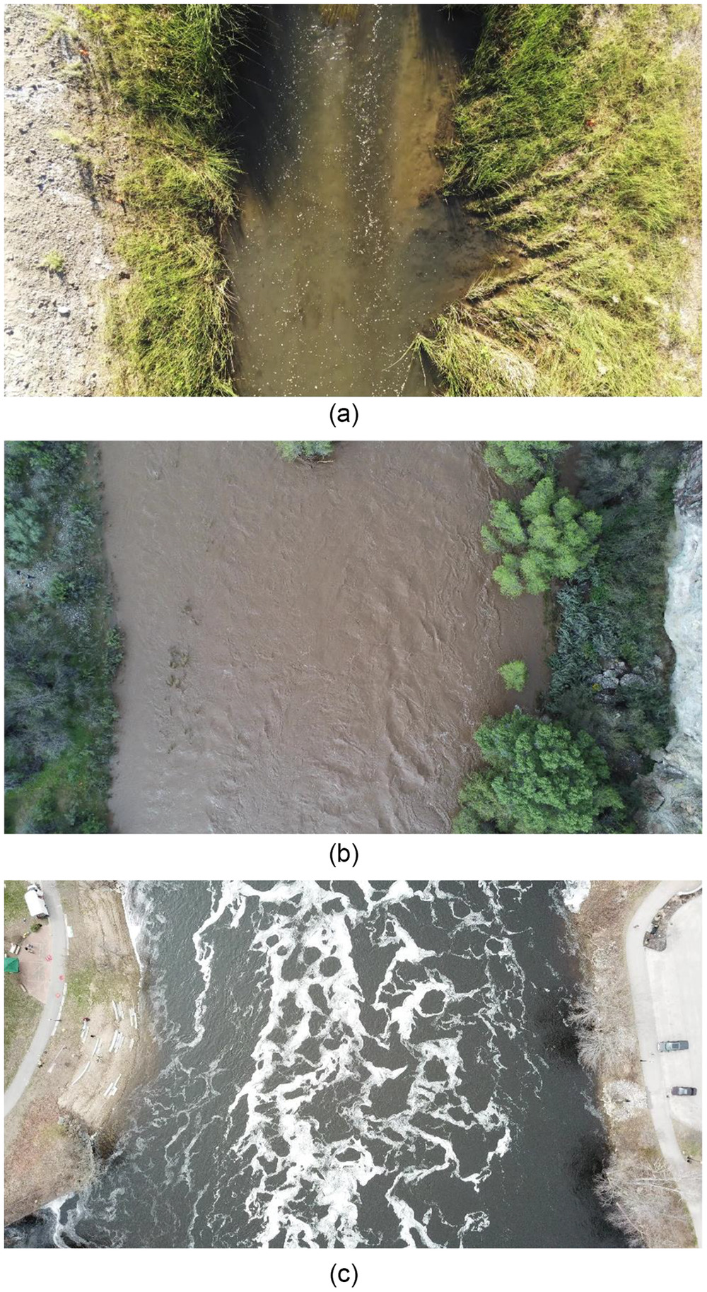
Eight field sites located in Arizona, New Mexico, California, and Maine were studied. A summary of site characteristics is presented in Table 1. Seven of the field sites were colocated with established USGS gauging stations. The Androscoggin River field site was located 2.8 km upstream of the nearest USGS gauging station. All but the Androscoggin River site are located in regions with typically flashy flood responses (Duan et al. 2017). The Wellton-Mohawk Main Outlet Drain (Fig. 1) is representative of what the other canal sites typically look like. The sUAS images in Fig. 2 show flow conditions during this study for the three natural river sites on the Agua Fria and Androscoggin Rivers.
| Channel name | Location | USGS site number | Type | Cross section | Drainage area () |
|---|---|---|---|---|---|
| Agua Fria River | Rock Springs, Arizona | 09512800 | Natural | Irregular | 2,874.9 |
| Androscoggin River | Auburn, Maine | 01059000 | Natural | Irregular | 7,536.9 |
| Gila River | Dome, Arizona | 09520500 | Natural | Irregular | 149,830.8 |
| Reservation Main Canal | Yuma, Arizona | 09523200 | Earthen | Trapezoidal | N/A |
| Wellton-Mohawk Main Outlet Drain | Yuma, Arizona | 09529300 | Concrete | Trapezoidal | N/A |
| Coachella Canal above All-American Canal Diversion | Felicity, California | 09527590 | Concrete | Trapezoidal | N/A |
| Cochiti East Side Main Canal | Cochiti, New Mexico | 08313500 | Concrete | Trapezoidal | N/A |
| Sile Main Canal (at Head) | Cochiti, New Mexico | 08314000 | Concrete | Rectangular | N/A |
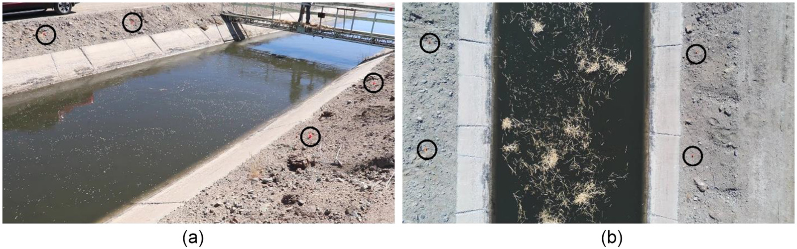
At each site, ground control points (GCPs) (e.g., solid circles in Fig. 1) were placed to calibrate the pixel ground scale resolution, which is required to translate pixel displacements computed from LSPIV into velocity units. The distances between the GCPs on each side of the channel were measured and recorded using either a tape measure or a laser rangefinder accurate to .
All sUAS video footage was collected with the camera pointing perpendicular to the water surface (nadir) with at least a 1 m of bank visible on each side. The sUAS pilot also ensured that at least two GCPs were visible and centered in the field of view of the camera. The flight altitude varied depending upon the channel width; for example, wider channels required the pilot to fly at a higher elevation so that the entire channel width including 1 m of bank on each side was visible in the field of view.
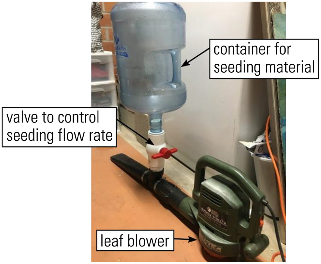
Seeding was necessary for applying the LSPIV algorithm in all but the Agua Fria and Androscoggin River sites. Both rice cereal and dry wheat straw were evaluated as seeding material. To uniformly distribute the rice cereal across the channel, a leaf blower was modified by cutting the blower hose and adding a valve to regulate the rate at which seeding material was dispersed (Fig. 3). Above the valve, a container to hold seeding material was installed. The blower functioned well, distributing seed material up to 15 m. Because the straw could not fit in the blower, it had to be spread by hand, and often formed clumps and dead areas where no seeding was visible. Seeding was best distributed across the channel when there was a bridge directly upstream of the measurement location, which allowed the leaf blower operator to stand directly over the middle of the channel and spray seeding back and forth across the entire channel width. Seeding from the channel banks led to inhomogeneous distribution of seeding across the channel.
Video footage from seven of the eight study sites was captured using a Parrot Anafi sUAS (Paris, France) shooting at at 30 frames per second (Anafi Parrot Drone 2021). The Androscoggin River field site used a Da Jiang innovations (DJI) Mavic Pro Government Edition drone shooting at at 24 frames per second to capture videos (DJI 2023). Video was collected for as long as wind and seeding conditions permitted (generally 20 to 30 s at a minimum).
To evaluate the sUAS derived methods in this study, flow velocities and discharge were measured at each field site at the time of sUAS data collection using either a Sontek M9 (San Diego) acoustic Doppler current profiler (ADCP) or Sontek Flowtracker operated by USGS hydrologists. Subsurface velocity data were collected either directly before or after video footage was captured with the sUAS. All ADCP data were postprocessed using Velocity Mapping Toolbox (VMT) version 4.09 (Parsons et al. 2013) to obtain the bathymetry and depth-averaged velocities. All discharge values measured by ADCP or acoustic Doppler velocimeter (ADV) were reviewed and processed using the QRev version 4.32 software application (Mueller 2020) according to current USGS policy (Turnipseed and Sauer 2010).
We treated the USGS reported discharge values as the truth reference values for evaluating the accuracies of sUAS derived discharges. The uncertainties of ADCP measured discharge at all sites were described by Engel et al. (2022) and are summarized in Table 3. In all but two cases (Table 3) the USGS reported quality was better than 9%. All input data for this study, including the sUAS videos, annotated images of GCP locations and distances, and subsurface velocity measurement files, are available (Engel et al. 2022).
Imagery Processing
This study used the Rectification of Image Velocity Results (RIVeR) toolbox version 2.5 (Patalano et al. 2017) to extract the frames from the video clips recorded from the sUAS and process LSPIV. To evaluate turbulent characteristics, all available frames were extracted because TDR relies on instantaneous velocity fluctuations. RIVeR uses an embedded version of PIVLab (Thielicke and Stamhuis 2014) to compute the time-resolved image velocimetry results. Image frame stabilization was performed using the approach of Farid and Woodward (2007), adapted to mask out the water (i.e., noncamera platform) motion from analysis in order to remove excess camera platform movement (e.g., the sUAS was not perfectly stable).
Each data set was preprocessed to enhance visualization of water surface seeding texture of the images. After conducting several trials and comparing the estimated surface velocities with the measured velocities from the ADCP, it was concluded that a contrast limited histogram equalization (CLAHE) with background subtraction produced the best particle tracking results. For all sites, a CLAHE window size of 20 pixels, corresponding to ground distances ranging from 0.04 to 0.73 m was used because the application of CLAHE was relatively insensitive to changes in window size.
A fast Fourier transform (FFT) multiwindow (three-pass) deformation PIV algorithm was utilized. Passes one, two, and three window sizes were set to ground distances ranging from 0.27 to 4.7 m (128 pixel), 0.13 to 2.35 m (64 pixel), and 0.07 to 1.17 m (32 pixel), respectively, depending on the site and pixel ground scale distances. These settings produced a displacement velocity vector at the center of each 32-pixel window in the region of interest, resulting in maximum vector spacings ranging from 0.067 m at the Sile Main Canal to 1.17 m at the Androscoggin River. Images were calibrated into real-world units using the GCPs. The output LSPIV analyses for each site comprised a time series of 2D surface velocities magnitudes () in the streamwise () and cross-stream () directions for each frame pair of the processed video. The time-series frequency was dictated by video framerate and ranged from 23.98 to 30 Hz (Engel et al. 2022).
Seeding Material Influence on Velocities
We compared seeding material influence on LSPIV velocity results to ADCP near-surface velocities at a cross section for the Wellton-Mohawk Main Outlet Drain site. The Wellton-Mohawk results shown in Fig. 4 are representatives of our findings, in which the root-mean square error (RMSE) using rice cereal, straw, and no seedings were 0.090, 0.094, and , and the corresponding normalized RMSE (NRMSE) were 9.26%, 9.67%, and 40.62%, respectively.

Nadir sUAS images at Reservation Main Canal illustrate the difference in surface texture between seeding material type (Fig. 5). Comparison of velocities by seeding material indicated that both straw and rice cereal are preferable with similar accuracy to no seeding material, but seeding is required in low-velocity, low-turbidity channels. For this reason, rice cereal was used because it was more economical and easier to distribute using the seeding distribution system (Fig. 3), except for the Gila and Androscoggin Rivers which were (1) too large to distribute seeding material across the measurement area, and (2) had better surface texture because of increased turbidity and velocity.

Computing Surface Turbulence Dissipation Rate from LSPIV Analysis
For each instantaneous velocity contained in the LSPIV-derived surface velocity time series (, ) along a given channel cross section, the streamwise () and transverse () fluctuations can be found by using Eqs. (1) and (2)where primes = instantaneous velocity fluctuations; overbars = time-averaging; and subscripts and th position along the cross section at the th time step. Assuming the turbulence flow is homogenous and isotropic, the TDR can be computed from the one-dimensional (1D) longitudinal () or transverse () velocity spectra from the velocities fluctuation expressed in 1D wave-number space, , whereand = wavelength. Based on Kolomogorov’s second similarity hypothesis, within the inertia subrange the statistics of motion are uniquely determined by the TDR, and the temporal energy spectra can be found as follows:where ; and , where and is TDR (Pope 2014). TDR was estimated by plotting the velocity spectra (, ) in the log space versus the wave number (Fig. 6), and taking the average of all spectra conforming to the best fit of a straight line with a slope of in the inertial subrange (i.e., the portion of the spectra in which or conforms to a slope line). Each line in Fig. 6 represents the results calculated from a time series of measured surface velocity at a transverse location in a section. The dissipation rate was averaged over several cross sections at a fixed transversal location. We found that in all sites, the streamwise velocity spectra were much wider in the inertia subrange than the transverse velocity spectra. The transverse spectra () tended to better follow the slope than the streamwise spectra (), the same as observed by Johnson and Cowen (2017a) in laboratory shallow open-channel flow experiments. Therefore, the transverse velocity spectra were selected for the estimation of turbulence dissipation rate for all further computations in this paper, consistent with the method used by Johnson and Cowen (2017a).
(1)
(2)
(3)
(4)
(5)

Calculating Friction Velocity
Nezu (1977) proposed a universal relation for the vertical distribution of turbulence dissipation in open-channel flows:where = turbulence energy dissipation rate at a location () along the th vertical; angled brackets = ensemble averaging; = friction velocity along the th vertical; and = flow depth at the th vertical in a cross section. Values of vary and typically range from 8.43 to as high as 13.4 (Pope 2014; Sukhodolov et al. 2006; Johnson and Cowen 2017a). We adopted the method of Johnson and Cowen (2017a) with by solving Eq. (5) for friction velocity using surface TDR (i.e., )
(6)
(7)
Furthermore, Johnson and Cowen (2017a) found that a constant ratio 1.24 between the near-surface and surface dissipation rate fit experimental data and provided a means to convert surface TDR into near-surface TDR. Although they rightly suggested further investigation is needed to confirm their laboratory results, we found good agreement in our observations (“Results” section). For our study, measured dissipation rates at the surface were converted to subsurface dissipation rates for each vertical in a cross section by multiplying by 1.24, and then Eq. (7) was applied to calculate the friction velocity, in which is set to 0.9.
Computing Depth-Averaged Velocities
We employed four methods to compute depth-averaged velocities: (1) constant-velocity index, (2) logarithmic velocity profile, (3) power-law profile, and (4) entropy method. Except for the entropy method, all the methods assumed a 1D velocity profile is valid for each vertical in each cross section. The following are detailed descriptions of each method.
Constant-Velocity Index
Hauet et al. (2018) studied over 3,000 individual discharge measurements to determine a constant-velocity index (). Their recommendations were to let equal 0.8 or 0.9 for mean flow depths greater or smaller 2.0 m, respectively and for concrete channels. We used a constant value of 0.80 at the Gila River () site, which had a maximum depth of 0.32 m (Table 2). The remaining study sites were assigned a value of 0.90 based on depth and channel type (Table 2). Depth-averaged velocities () were then computed as follows:where = surface velocity determined by LSPIV at the th vertical.
(8)
| Channel name | Width (m) | Maximum depth (m) | Average velocity () | Maximum velocity () | Mean annual flow () | ADCP measured discharge | |
|---|---|---|---|---|---|---|---|
| Discharge () | Uncertainty (%) | ||||||
| Agua Fria River | 65.00 | 3.04 | 2.40 | N/A | 2.31 | 255.51 | 20.0 |
| Androscoggin River | 99.20 | 6.70 | 0.89 | 1.68 | 0.00 | 410.23 | 8.4 |
| Gila River | 3.66 | 0.32 | 0.24 | 0.45 | 6.68 | 0.17 | 4.0 |
| Reservation Main Canal | 10.80 | 1.10 | 0.19 | 0.37 | 2.04 | 1.70 | 4.4 |
| Wellton-Mohawk Main Outlet Drain | 5.63 | 1.18 | 0.91 | 1.25 | 5.86 | 4.13 | 5.5 |
| Coachella Canal | 12.91 | 2.76 | 0.81 | 1.48 | 12.60 | 21.44 | 4.6 |
| Cochiti East Side Main Canal | 6.82 | 1.38 | 0.49 | 0.74 | 0.00 | 2.86 | 19.5 |
| Sile Main Canal (at Head) | 1.83 | 1.10 | 0.80 | 0.94 | 0.00 | 1.44 | 8.0 |
Note: Site characteristics, velocity, and mean annual and measured discharge data are from USGS (2023).
Logarithmic Velocity Profile
The depth-averaged logarithmic velocity profile for open-channel flow can be expressedwhere = depth at vertical ; is the Von Karman’s constant; and = characteristic roughness height. Eq. (9) is valid in the inner layer of rough bed flows in the range (Smart 1999). The roughness height is several times (e.g., , , and ) of the median diameter of homogenous sand particles (Monin and Yaglom 1971; Townsend 1976). A wide range of roughness height is expected in rough bed flows depending on bed sediment and irregularities of bed surface. At field sites in this study, the size of bed sediment was unknown; thus, the roughness height was treated as an unknown parameter equal to a fraction of local flow depth as . This assumption was derived from the experimental study of over gravel bed surfaces, in which was found to be linearly proportional to bed shear stress in uniform flow (Smart 1999). The bed shear stress in uniform flow is linearly proportional to flow depth, therefore, the ratio of is a constant for uniform flow. Flow was nearly steady uniform at the study sites, which validates this assumption. Optimal values were selected at each site by using trial and error for ranging from 0.001 to 0.02. Chosen values of value and the corresponding error of discharge estimation are summarized in Table 3. Options for cases where the optimization of with the existing measurements is not possible are discussed more in the “Results” section.
(9)
| Channel name | Location | Measured discharge | Constant-velocity index | Power-law | value in | Log law | Log-wake law | Entropy method | |
|---|---|---|---|---|---|---|---|---|---|
| Discharge () | Uncertainty (%) | ||||||||
| Agua Fria River | Rock Springs, Arizona | 255.51 | 20.0 | 265.71 | 179.50 | 0.063 | 254.17 | 282.97 | 299.69 |
| Androscoggin River | Auburn, Maine | 410.23 | 8.4 | 409.67 | 293.92 | 0.068 | 414.16 | 463.23 | 558.70 |
| Gila River | Dome, Arizona | 0.17 | 4.0 | 0.15 | 0.14 | 0.072 | 0.18 | 0.20 | 0.32 |
| Reservation Main Canal | Yuma, Arizona | 1.70 | 4.4 | 1.48 | 1.65 | 0.100 | 1.71 | 1.97 | 2.01 |
| Wellton-Mohawk Main Outlet Drain | Yuma, Arizona | 4.13 | 5.5 | 3.29 | 2.17 | 0.003 | 4.25 | 4.43 | 3.90 |
| Coachella Canal | Felicity, California | 21.44 | 4.6 | 18.25 | 11.28 | 0.007 | 21.35 | 22.43 | 20.77 |
| Cochiti East Side Main Canal | Cochiti, New Mexico | 2.86 | 19.5 | 2.20 | 2.18 | 0.040 | 2.77 | 3.02 | 2.87 |
| Sile Main Canal (at Head) | Cochiti, New Mexico | 1.44 | 8.0 | 1.26 | 0.86 | 0.007 | 1.44 | 1.51 | 1.57 |
Note: The method with the closest prediction for each site is in bold.
To compensate the deviation from the logarithmic velocity profile as , a wake coefficient can be added to Eq. (9). The depth-averaged velocity using the log-wake velocity profile is written
(10)
The value of in Eq. (10) is dependent on the Reynolds number (), in which is the kinematic viscosity of water. For a low Reynolds number (), ; at a high Reynolds number (), (Nezu and Rodi 1986; Lyn 1988).
Power-Law Velocity Profile
The velocity distribution can also be approximated with a power-law velocity profile at each vertical of the formwhere = power exponential; and = maximum velocity at water surface at the th vertical. Integrating Eq. (11), depth-averaged mean velocity can be calculated as follows:
(11)
(12)
The exponential depends on Reynolds number and bed roughness (Sturm 2021). Johnson and Cowen (2017b) redefined the skin friction factor in terms of surface velocity as . Applying the boundary layer flow theory and setting the Clauser shape factor for the rough bed case, the shape factor can be written as , in which is equal to the ratio of the displacement thickness to the momentum thickness in a boundary layer flow (Johnson and Cowen 2017b). From this, can be expressed as a function of the shape factor
(13)
Eq. (13) requires to produce a positive . In cases where friction velocity is much lower than surface velocity () such as may occur in smooth and/or deep flows, can approach 1.0 and approaches infinity, suggesting the depth-averaged velocity is nearly equal to the surface velocity. To solve for depth-averaged velocities, the friction velocity () and surface velocity () at each vertical are used with Johnson and Cowen’s (2017b) method to determine the drag coefficient () and parameter, which is then used to solve Eqs. (12) and (13).
Entropy Method
The previous three methods are based on a 1D velocity distribution. The entropy method applies the 2D velocity distribution derived from Shannon’s entropy theory (Chiu 1987, 1988). Chiu (1988) first derived the 2D velocity distribution for open-channel flow as follows:where = velocity at a given location () in a cross section; = entropy parameter measuring the uniformity of the velocity distribution; and = dimensionless coordinate, in which , , and = isovels of velocity equal to 0, , and , respectively. Chiu (1988) found is dependent on the friction factor and Reynold number, and for natural channels of erodible boundary, the value of typically ranges from 7 to 8. Chiu (1991) assumed the probability function of velocity occurring in a cross section as follows:where = probability density function of velocity; and and = parameters that can be solved by maximizing the Shannon entropy to the constraints described by Chiu (1991). Using the shear velocity at the channel boundary, the parameter can be solved as follows:where is the average integral constant of on the channel boundary; = representative averaged shear velocity for the cross section; andwhere = vertical distance from the location of maximum velocity to the water surface. If , then and , therefore, Eq. (16) can be simplified as follows:
(14)
(15)
(16)
(17)
(18)
Chiu (1991) found the parameter can be determined from and directly as follows [Eq. (16) in Chiu (1991)]:
(19)
In this study, the maximum surface velocity in the cross section was denoted as , and we assumed the maximum velocity at the surface is the maximum for the cross section (i.e., ), which may or may not be true for each site. Then, was calculated using the Nezu (1977) general relation [Eq. (7)] using . The averaged friction velocity () was calculated as the root-mean square of for all verticals in each cross section, and flow depth was taken as hydraulic depth, which is equal to the flow area divided by the top width. Then, the cross-sectional mean velocity () was calculated as follows:
(20)
Computing Discharge
When applying the constant-velocity index, the logarithmic law and the power-law methods, the depth-averaged velocity was calculated for each vertical and the total discharge is the summation of all the subdischarges according to the mean-section methodwhere = number of subsections in a cross section; and = distance between the verticals and . Discharge was computed from the entropy method as the product of cross-sectional mean velocity determined by Eq. (20) and cross-sectional area
(21)
(22)
Results
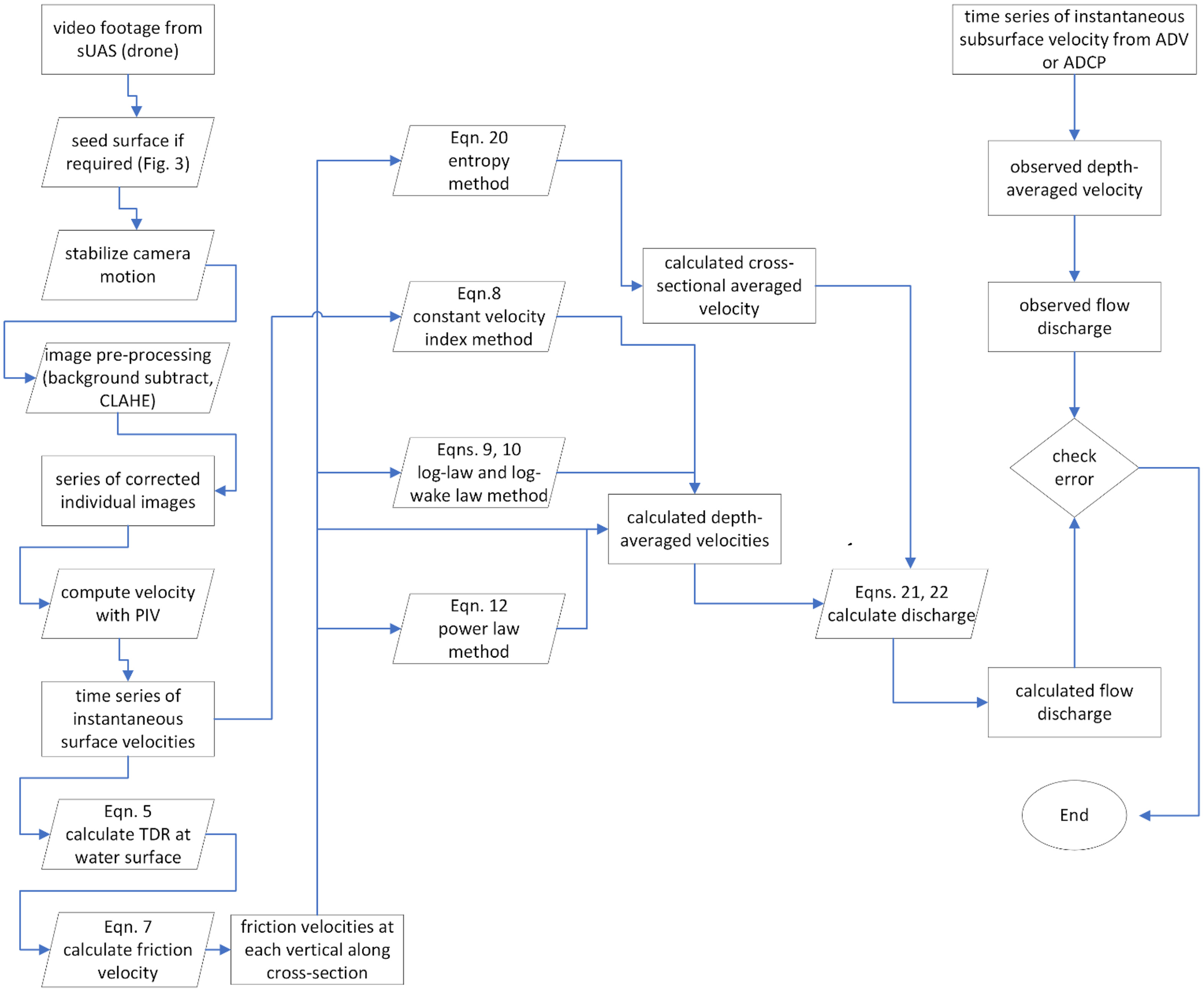
A flowchart summarizing the process of computing discharge for each method, labeled with the key equations used in each step, is shown in Fig. 7. Table 3 summarizes the estimated discharges from the four methods and the corresponding conventionally measured discharges, which were considered truth for evaluation purposes. The normalized errors of estimated discharges were calculated from the estimated () and the observed () discharges as , and are summarized in Table 4 together with the channel types and ratios. For each field site, the estimated discharges are reported by method, and the methods with the least normalized error are in bold.
| Channel name | Type | Width to depth ratio | Constant-velocity index (%) | Power-law (%) | value in | Log law (%) | Log-wake law (%) | Entropy method (%) |
|---|---|---|---|---|---|---|---|---|
| Agua Fria River | Natural | 21.54 | 3.99 | 29.75 | 0.063 | 0.53 | 10.75 | 17.29 |
| Androscoggin River | Natural | 15.22 | 0.14 | 28.35 | 0.068 | 0.96 | 12.92 | 36.19 |
| Gila River | Natural | 10.4 | 15.14 | 20.54 | 0.072 | 2.50 | 15.07 | 83.09 |
| Reservation Main Canal | Earthen | 10.57 | 13.07 | 3.41 | 0.100 | 0.03 | 15.39 | 18.15 |
| Wellton-Mohawk Main Outlet Drain | Concrete | 4.37 | 20.38 | 47.34 | 0.003 | 3.01 | 7.29 | 5.68 |
| Coachella Canal above All-American Canal Diversion | Concrete | 4.46 | 14.88 | 47.36 | 0.007 | 0.38 | 4.64 | 3.13 |
| Cochiti East Side Main Canal | Concrete | 4.44 | 23.25 | 23.69 | 0.040 | 3.15 | 5.58 | 0.47 |
| Sile Main Canal (at Head) | Concrete | 1.64 | 12.00 | 40.20 | 0.007 | 0.36 | 5.43 | 9.33 |
Note: The method with the lowest normalized error for each site is in bold.
When applying the logarithmic law profile, a roughness height needs to be selected in Eqs. (9) and (10). Because bed sediment size was not available, the was assumed to be proportional to local flow depth as , where was optimized using field measurements and varied from 0.04 to 0.1, which is consistent with other research (Bagherimiyab and Lemmin 2013). Because Eq. (9) is theoretically only valid to due to free surface effects, the log-wake law [Eq. (10)] was also evaluated. However, the log-law without wake correction performed better than the log-wake law at all sites in this study (Table 4).
Moreover, the log-law estimated discharges at the four sites with —including three natural rivers and one earthen canal—performed best relative to the other sites with . At the four sites with the values of were relatively uniform with an average of 0.076 (, , and ). However, at the sites with , the values of were less uniform with an average of 0.014 (, , and ). This suggests the log-law method may be more accurate for estimating the depth-averaged velocity for presuming can be optimized with known discharge reference data.
The results from the power-law method were not as accurate as the either log-law method (Table 4), and values of at multiple verticals at the Androscoggin, Reservation Main and Cochiti East Side Main Canal sites were less than 1.0, leading to , which is nonsensical. Thus, the depth-averaged velocity was assumed equal to the observed surface velocity for these cases. The power-law profile performed best at Reservation Main Canal Site (3.41% error), but all other sites had larger reported percent errors (Table 4). We suspect that the computed skin friction factor () based on surface velocities performed poorly owing to the assumption that there was no form drag present (Johnson and Cowen 2017b). Calibration of and further evaluation of the empirical relation between and could be re-examined as more laboratory and field data become available.
For the entropy method, we assumed the maximum velocity occurred at the free surface, and the observed maximum velocity at surface was the maximum velocity in the entire cross section. The entropy method performed best for the concrete canal sites with . However, at the Sile Main Canal (), flow was noted in the field to be 2D, and the maximum velocity likely occurred below the water surface, violating our assumptions and increasing the percent error of discharges at this site to a higher value (9.33%) relative to the other sites with . Estimated discharges using the logarithmic law method [Eq. (9)] were much more accurate than the discharges computed from the entropy method for the sites where .
The constant-velocity index method performed best at the Androscoggin River site (0.14% error) (Tables 4 and 5). However, the absolute errors at the four sites with ranged from 0.14% to 15.14%. At the other four sites, , and the errors ranged from 12.00% to 23.25%. When comparing with the results from the entropy method, the constant-velocity index method was more accurate than the entropy method for , but less than accurate for .
| Channel name | Width and depth ratio | Constant-velocity index (%) | Entropy method (%) | value | Log law (%) | Log-wake law (%) | value | Log law (%) | Log-wake law (%) |
|---|---|---|---|---|---|---|---|---|---|
| Agua Fria River | 3.99 | 17.29 | 11.10 | 0.17 | |||||
| Androscoggin River | 0.14 | 36.19 | 5.69 | 6.27 | |||||
| Gila River | 15.14 | 83.09 | 0.90 | 11.67 | |||||
| Reservation Main Canal | 13.07 | 18.15 | 21.11 | 36.46 | |||||
| Wellton-Mohawk Main Outlet Drain | 20.38 | 5.68 | 29.99 | 25.70 | 15.14 | 10.86 | |||
| Coachella Canal Diversion | 14.88 | 3.13 | 17.81 | 12.78 | 0.38 | 4.64 | |||
| Cochiti East Side Main Canal | 23.25 | 0.47 | 42.68 | 51.41 | 72.93 | 81.66 | |||
| Sile Main Canal (at Head) | 12.00 | 9.33 | 17.20 | 12.13 | 0.36 | 5.43 |
Note: Bold numbers are satisfactory results.
Discussion
Based on results from the eight field sites studied here, the log-law, constant-velocity index, and the entropy method performed best at estimating discharge from measured surface velocity and TDR. The most accurate results from this study were achieved using the log-law or log-wake-law approach with the value calibrated to roughness values at each site. By summarizing the results of optimization of the parameter, we find it may be possible to select values without any precalibration. The average of precalibrated values for the sites in this study having (Table 4) was 0.076, corresponding to a roughness height . Similarly, for (Table 4) at the four concrete canal sites, the constant values were 0.003, 0.007, 0.04, and 0.07, with average and median values of 0.014 and 0.007, respectively.
Discharge was recomputed using the summarized values of for each site based on (Table 5). When choosing for , the largest error was 21.11% at the Reservation Main Canal, and the errors at other three sites ranged from 0.9% to 11.1%. These errors were smaller than the results using the entropy method but larger than the errors using the constant-velocity index method at three of the four sites, indicating that for natural rivers with , the constant-velocity index method is more accurate than the log-law or log-wake law methods regardless when selecting a constant .
For , errors using the entropy method were smaller than either the average value of or the constant-velocity index methods. Without knowing in log-law or log-wake law, the results suggest the constant-velocity index method performed the best for natural rivers of , whereas the entropy method was the best for concrete canals with . Based on our results, should be used for the log-law method for natural rivers of . The log-law method may not yield accurate results when using or for concrete canals.
Conclusions
This study evaluated the methods of river discharge estimation using videos recorded by sUAS at eight unique field sites. Of the eight study sites, four were engineered concrete channels, three were natural channels, and one was an engineered earthen channel. Each of these sites differed in channel geometry, flow, and seeding characteristics. With the instantaneous and average surface velocity distributions computed from LSPIV at each site, the TDR was estimated from 1D transverse velocity spectra for calculating the friction velocity. Depth-averaged velocity was calculated using four methods: the constant-velocity index, the logarithmic law (with or without wake correction), the power-law, and the entropy method. From our findings, these general recommendations emerged:
•
For sites with where the flow could be approximated as 1D () the logarithmic law method without wake correction using a calibrated roughness height was the most accurate.
•
The best results were found by calibrating the roughness parameter as a function of depth () using field measurements. Without field measurement calibration, the best results were obtained by for and in concrete channels (results for other channel types were not accurate).
•
For sites with without a priori knowledge of boundary roughness conditions, the entropy method produced the best results.
•
For sites with without a priori knowledge of boundary roughness conditions, the constant-velocity index method was the most accurate, but the logarithmic law method with also performed adequately.
One should select the best approach for velocity calculations using ratios and channel types. The recommended value for is based on the data from these eight sites, and the maximum error can be as high as 21.11%. Additional field data are needed to verify if is the most suitable value for using the log-law.
This study did not evaluate sites with , and thus does not draw conclusions about this range. More research is needed to search for and evaluate approaches to precalibrate the roughness parameter used in the logarithmic law method and to include sites of medium ratios. Although limited in scope, this research shows that under ideal seeding and flow conditions, discharge can be accurately calculated from TDR and surface flow velocities obtained from the images collected remotely.
Notation
The following symbols are used in this paper:
- channel area;
- ,
- parameters used in the maximization of Shannon entropy;
- distance between verticals in a cross section;
- ,
- constants associated with the Kolomogorov similarity hypothesis;
- skin friction factor;
- median grain size of sediment;
- empirical constant derived by Nezu (1977) used in the universal relation of the vertical distribution of turbulence dissipation;
- ,
- longitudinal and transverse velocity spectra, respectively;
- Clauser shape factor;
- shape factor;
- flow depth;
- vertical distance from the location of maximum cross-sectional velocity to the water surface;
- ,
- th position along a cross section at the th time step;
- entropy parameter;
- power exponential used in the power-law method;
- number of subsections in a cross section;
- probability density function of velocities within a cross section;
- flow discharge;
- Reynolds number;
- ,
- streamwise and cross-stream velocity, respectively;
- ,
- instantaneous streamwise and cross-stream velocity, respectively;
- shear velocity;
- streamwise cross-sectional maximum velocity;
- streamwise cross-sectional mean velocity;
- streamwise surface velocity;
- vertical position between the bed and flow depth;
- characteristic roughness height;
- constant-velocity index;
- turbulent dissipation rate;
- Von Karman constant;
- one-dimensional wave-number space;
- wavelength;
- kinematic viscosity of water;
- dimensionless coordinate along rays used in the entropy method;
- dimensionless isovel of velocity at ;
- dimensionless isovel of velocity at ; and
- Cole’s wake coefficient.
Data Availability Statement
The original video recordings at eight sites are published in accordance with the USGS data retention policy online (Engel et al. 2022). The Python program for calculating discharge using methods described in the paper is also published by the University of Arizona data repository (Duan et al. 2022). Other data (e.g., RIVeR software) that support the findings of this study are available from the corresponding author upon reasonable request.
Acknowledgments
This research is funded by USGS Water Resource Research Center 104B Grant to the University of Arizona. USGS personnel in the Yuma, Arizona, and Albuquerque, New Mexico, field offices have provided all the ADCP and Flowtracker velocity data for matching the data collected by the sUAS. We are grateful to the funding support and technical assistance from USGS. Any use of trade, firm, or product names is for descriptive purposes only and does not imply endorsement by the US Government.
References
Anafi Parrot Drone. 2021. “Anafi user guide version 6.7.0.1.” Accessed August 3, 2023. https://www.parrot.com/assets/s3fs-public/2021-09/anafi-user-guide.pdf.
Bagherimiyab, F., and U. Lemmin. 2013. “Shear velocity estimates in rough-bed open-channel flow.” Earth Surf. Processes Landforms 38 (14): 1714–1724. https://doi.org/10.1002/esp.3421.
Bandini, F., B. Lüthi, S. Peña-Haro, C. Borst, J. Liu, S. Karagkiolidou, X. Hu, G. G. Lemaire, P. L. Bjerg, and P. Bauer-Gottwein. 2021. “A drone-borne method to jointly estimate discharge and manning’s roughness of natural streams.” Water Resour. Res. 57 (2): e2020WR028266. https://doi.org/10.1029/2020WR028266.
Bjerklie, D. M., J. W. Fulton, S. L. Dingman, M. G. Canova, J. T. Minear, and T. Moramarco. 2020. “Fundamental hydraulics of cross sections in natural rivers: Preliminary analysis of a large data set of acoustic Doppler flow measurements.” Water Resour. Res. 56: e2019WR025986. https://doi.org/10.1029/2019WR025986.
Bradley, A. A., A. Kruger, E. A. Meselhe, and M. V. Muste. 2002. “Flow measurement in streams using video imagery.” Water Resour. Res. 38 (12): 1–8. https://doi.org/10.1029/2002WR001317.
Chiu, C. 1987. “Entropy and probability concepts in hydraulics.” J. Hydraul. Eng. 113 (5): 583–599. https://doi.org/10.1061/(ASCE)0733-9429(1987)113:5(583).
Chiu, C. 1988. “Entropy and 2-D velocity distribution in open channels.” J. Hydraul. Eng. 114 (7): 738–756. https://doi.org/10.1061/(ASCE)0733-9429(1988)114:7(738).
Chiu, C. L. 1991. “Application of entropy concept in open-channel flow study.” J. Hydraul. Eng. 117 (5): 615–628. https://doi.org/10.1061/(ASCE)0733-9429(1991)117:5(615).
Chiu, C. L., and N. C. Tung. 2002. “Maximum velocity and regularities in open-channel flow.” J. Hydraul. Eng. 128 (4): 390–398. https://doi.org/10.1061/(ASCE)0733-9429(2002)128:4(390).
Creutin, J. D., M. Muste, A. A. Bradley, S. C. Kim, and A. Kruger. 2003. “River gauging using PIV techniques: A proof of concept experiment on the Iowa River.” J. Hydrol. 277 (3–4): 182–194. https://doi.org/10.1016/S0022-1694(03)00081-7.
Dal Sasso, S. F., A. Pizarro, and S. Manfreda. 2020. “Metrics for the quantification of seeding characteristics to enhance image velocimetry performance in rivers.” Remote Sens. 12 (11): 1789. https://doi.org/10.3390/rs12111789.
DJI (Da Jiang Innovations). 2023. “Mavic Pro—Product information website.” Accessed August 3, 2023. https://www.dji.com/mavic/info#specs.
Duan, J. G., Y. Bai, F. Dominguez, E. Rivera, and T. Meixner. 2017. “Framework for incorporating climate change on flood magnitude and frequency analysis in the upper Santa Cruz River.” J. Hydrol. 549 (Jun): 194–207. https://doi.org/10.1016/j.jhydrol.2017.03.042.
Duan, J. G., A. Cadogan, and F. L. Engel. 2022. Data for field application of turbulence energy dissipation rate for estimating flow discharge. Tucson, AZ: Univ. of Arizona. https://doi.org/10.25422/azu.data.21114139.v1.
Engel, F. L., A. Cadogan, and J. D. Duan. 2022. Small unoccupied aircraft system imagery and associated data used for discharge measurement at eight locations across the United States in 2019 and 2020. Washington, DC: USGS. https://doi.org/10.5066/P9H2MM1M.
Farid, H., and J. B. Woodward. 2007. “Video stabilization and enhancement.” Accessed August 3, 2023. https://digitalcommons.dartmouth.edu/cs_tr/305.
Farina, G., S. Alvisi, M. Franchini, and T. Moramarco. 2014. “Three methods for estimating the entropy parameter M based on a decreasing number of velocity measurements in a river cross-section.” Entropy 16 (5): 2512–2529. https://doi.org/10.3390/e16052512.
Fujita, I., M. Muste, and A. Kruger. 1998. “Large-scale particle image velocimetry for flow analysis in hydraulic engineering applications.” J. Hydraul. Res. 36 (3): 397–414. https://doi.org/10.1080/00221689809498626.
Fulton, J., and J. Ostrowski. 2008. “Measuring real-time streamflow using emerging technologies: Radar, hydroacoustics, and the probability concept.” J. Hydrol. 357 (1–2): 1–10. https://doi.org/10.1016/j.jhydrol.2008.03.028.
Fulton, J. W., et al. 2020a. “QCam: sUAS-based doppler radar for measuring river discharge.” Remote Sens. 12 (20): 3317. https://doi.org/10.3390/rs12203317.
Fulton, J. W., et al. 2020b. “Near-field remote sensing of surface velocity and river discharge using radars and the probability concept at 10 U.S. Geological Survey streamgages.” Remote Sens. 12 (8): 1296. https://doi.org/10.3390/rs12081296.
Guillén, N. F., A. Patalano, C. M. García, and J. C. Bertoni. 2017. “Use of LSPIV in assessing urban flash flood vulnerability.” Nat. Hazards 87: 383–394. https://doi.org/10.1007/s11069-017-2768-8.
Hauet, A., T. Morlot, and L. Daubagnan. 2018. “Velocity profile and depth-averaged to surface velocity in natural streams: A review over a large sample of rivers.” In Vol. 40 of Proc., River Flows 2018—Ninth Int. Conf. on Fluvial Hydraulics, 06015. Les Ulis Cedex, France: EDS Science. https://doi.org/10.1051/e3sconf/20184006015.
Huang, H., D. Dabiri, and M. Gharib. 1997. “On errors of digital particle image velocimetry.” Meas. Sci. Technol. 8 (12): 1427–1440. https://doi.org/10.1088/0957-0233/8/12/007.
Hulsing, H., W. Smith, and E. D. Cobb. 1966. Velocity-head coefficients in open channels. Washington, DC: US Government Printing Office.
Jin, T., and Q. Liao. 2019. “Application of large scale PIV in river surface turbulence measurements and water depth estimation.” Flow Meas. Instrum. 67 (4): 142–152. https://doi.org/10.1016/j.flowmeasinst.2019.03.001.
Jodeau, M., A. Hauet, A. Paquier, J. Le Coz, and G. Dramais. 2008. “Application and evaluation of LS-PIV technique for the monitoring of river surface velocities in high flow conditions.” Flow Meas. Instrum. 19 (2): 117–127. https://doi.org/10.1016/j.flowmeasinst.2007.11.004.
Johnson, E. D., and E. A. Cowen. 2017a. “Estimating bed shear stress from remotely measured surface turbulent dissipation fields in open channel flows.” Water Resour. Res. 53 (3): 1982–1996. https://doi.org/10.1002/2016WR018898.
Johnson, E. D., and E. A. Cowen. 2017b. “Remote determination of the velocity index and mean streamwise velocity profiles.” Water Resour. Res. 53 (9): 7521–7535. https://doi.org/10.1002/2017WR020504.
Keane, R. D., and R. J. Adrian. 1992. “Theory of cross-correlation analysis of PIV images.” Appl. Sci. Res. 49 (3): 191–215. https://doi.org/10.1007/BF00384623.
Le Coz, J., et al. 2016. “Crowd-sourced data for flood hydrology: Feedback from recent citizen science projects in Argentina, France and New Zealand.” J. Hydrol. 541 (Oct): 766–777. https://doi.org/10.1016/j.jhydrol.2016.07.036.
Legleiter, C. J., P. J. Kinzel, and J. M. Nelson. 2017. “Remote measurement of river discharge using thermal particle image velocimetry (PIV) and various sources of bathymetric information.” J. Hydrol. 554 (Nov): 490–506. https://doi.org/10.1016/j.jhydrol.2017.09.004.
Lewis, Q. W., E. M. Lindroth, and B. L. Rhoads. 2018. “Integrating unmanned aerial systems and LSPIV for rapid, cost-effective stream gauging.” J. Hydrol. 560 (May): 230–246. https://doi.org/10.1016/j.jhydrol.2018.03.008.
Lewis, Q. W., and B. L. Rhoads. 2015. “Resolving two-dimensional flow structure in rivers using large-scale particle image velocimetry: An example from a stream confluence.” Water Resour. Res. 51 (10): 7977–7994. https://doi.org/10.1002/2015WR017783.
Lyn, D. 1988. “A similarity approach to turbulent sediment-laden flows in open channels.” J. Fluid Mech. 193 (Aug): 1–26. https://doi.org/10.1017/S0022112088002034.
Monin, A. S., and A. M. Yaglom. 1971. Vol. I of Statistical fluid mechanics. Cambridge, MA: MIT Press.
Moramarco, T., S. Barbetta, and A. Tarpanelli. 2017. “From surface flow velocity measurements to discharge assessment by the entropy theory.” Water 9 (2): 120. https://doi.org/10.3390/w9020120.
Moramarco, T., C. Saltalippi, and V. P. Singh. 2004. “Estimation of mean velocity in natural channel based on Chiu’s velocity distribution equation.” J. Hydrol. Eng. 9 (1): 42–50. https://doi.org/10.1061/(ASCE)1084-0699(2004)9:1(42).
Moramarco, T., and V. P. Singh. 2010. “Formulation of the entropy parameter based on hydraulic and geometric characteristics of river cross sections.” J. Hydrol. Eng. 15 (10): 852–858. https://doi.org/10.1061/(ASCE)HE.1943-5584.0000255.
Mueller, D. S. 2020. QRev. US Geological Survey software release. Washington, DC: USGS. https://doi.org/10.5066/P9OZ8QDL.
Nezu, I. 1977. “Turbulent structure in open-channel flows.” Ph.D. dissertation, Dept. of Engineering, Kyoto Univ.
Nezu, I., and W. Rodi. 1986. “Open-channel flow measurements with a Laser Doppler anemometer.” J. Hydraul. Eng. 112 (5): 335–355. https://doi.org/10.1061/(ASCE)0733-9429(1986)112:5(335).
Parsons, D. R., P. R. Jackson, J. A. Czuba, F. L. Engel, B. L. Rhoads, K. A. Oberg, J. L. Best, D. S. Mueller, K. K. Johnson, and J. D. Riley. 2013. “Velocity mapping toolbox (VMT): A processing and visualization suite for moving-vessel ADCP measurements.” Earth Surf. Processes Landforms 38 (11): 1244–1260. https://doi.org/10.1002/esp.3367.
Patalano, A., C. M. García, and A. Rodríguez. 2017. “Rectification of image velocity results (RIVeR): A simple and user-friendly toolbox for large scale water surface particle image velocimetry (PIV) and particle tracking velocimetry (PTV).” Comput. Geosci. 109 (Dec): 323–330. https://doi.org/10.1016/j.cageo.2017.07.009.
Pearce, S., et al. 2020. “An evaluation of image velocimetry techniques under low flow conditions and high seeding densities using unmanned aerial systems.” Remote Sens. 12 (2): 232. https://doi.org/10.3390/rs12020232.
Perks, M. T., S. F. Dal Sasso, A. Hauet, J. Le Coz, S. Pearce, S. Peña-Haro, F. Tauro, J. Bomhof, and S. Grimaldi. 2020. “Towards harmonization of image velocimetry techniques for river surface velocity observations.” Earth Syst. Sci. Data 12 (3): 1545–1559. https://doi.org/10.5194/essd-12-1545-2020.
Perks, M. T., A. J. Russell, and A. R. G. Large. 2016. “Technical note: Advances in flash flood monitoring using unmanned aerial vehicles (UAVs).” Hydrol. Earth Syst. Sci. 20 (10): 4005–4015. https://doi.org/10.5194/hess-20-4005-2016.
Pizarro, A., S. F. Dal Sasso, M. T. Perks, and S. Manfreda. 2020. “Identifying the optimal spatial distribution of tracers for optical sensing of stream surface flow.” Hydrol. Earth Syst. Sci. 24: 5173–5185. https://doi.org/10.5194/hess-24-5173-2020.
Polatel, C. 2005. “Indexing by free surface velocity: A prospect for remote discharge estimation.” In Proc., 31st IAHR Congress 2005: Water Engineering for the Future, Choices and Challenges, 6552–6559. Beijing: IAHR Secretariat.
Pope, S. B. 2014. Turblent flows. Cambridge, UK: Cambridge University Press.
Rantz, S. E. 1982. Measurement and computation of streamflow. Vol. 1—Measurement of stage and discharge. Denver: USGS.
Smart, G. M. 1999. “Turbulent velocity profiles and boundary shear in gravel bed rivers.” J. Hydraul. Eng. 125 (2): 106–116. https://doi.org/10.1061/(ASCE)0733-9429(1999)125:2(106).
Sturm, T. 2021. Open channel hydraulics. New York: McGraw Hill.
Sukhodolov, A. N., J. J. Fedele, and B. L. Rhoads. 2006. “Structure of flow over alluvial bedforms: An experiment on linking field and laboratory methods.” Earth Surf. Processes Landforms 31 (10): 1292–1310. https://doi.org/10.1002/esp.1330.
Tauro, F., A. Petroselli, and E. Arcangeletti. 2016. “Assessment of drone-based surface flow observations.” Hydrol. Processes 30 (7): 1114–1130. https://doi.org/10.1002/hyp.10698.
Thielicke, W., and E. J. Stamhuis. 2014. “PIVlab—Towards user-friendly, affordable and accurate digital particle image velocimetry in MATLAB.” J. Open Res. Software 2 (1): e30. https://doi.org/10.5334/jors.bl.
Townsend, A. A. 1976. The structure of turbulence shear flow. Cambridge, UK: Cambridge University Press.
Turnipseed, D. P., and V. B. Sauer. 2010. Discharge measurements at gaging stations. Denver: USGS.
USGS. 2023. “National Water Information System data (Water Data for the Nation).” Accessed August 3, 2023. http://waterdata.usgs.gov/nwis/.
Information & Authors
Information
Published In

Journal of Hydraulic Engineering
Volume 149 • Issue 11 • November 2023
Copyright
This work is made available under the terms of the Creative Commons Attribution 4.0 International license, https://creativecommons.org/licenses/by/4.0/.
History
Received: Nov 29, 2022
Accepted: Jun 4, 2023
Published online: Sep 15, 2023
Published in print: Nov 1, 2023
Discussion open until: Feb 15, 2024
ASCE Technical Topics:
- Aerodynamics
- Aerospace engineering
- Aircraft and spacecraft
- Computer vision and image processing
- Continuum mechanics
- Dynamics (solid mechanics)
- Engineering fundamentals
- Engineering mechanics
- Flow (fluid dynamics)
- Flow measurement
- Fluid dynamics
- Fluid mechanics
- Fluid velocity
- Hydrologic engineering
- Measurement (by type)
- Methodology (by type)
- Overland flow
- Particle velocity
- Solid mechanics
- Water and water resources
- Water discharge
- Water discharge measurement
Authors
Metrics & Citations
Metrics
Citations
Download citation
If you have the appropriate software installed, you can download article citation data to the citation manager of your choice. Simply select your manager software from the list below and click Download.