Abstract
Resuspension and redistribution of sediments induced by propeller wash may significantly influence aquatic ecosystems at contaminated sediment sites. This study describes a numerical modeling method developed to predict the sediment resuspension and subsequent transport processes resulting from ship traffic, with a fully coupled simulation of hydrodynamics, sediment transport, and propeller wash. By including propeller momentum effects in the flow field computation, the advection and dispersion of resuspended sediments are better represented than in previously available methods. To achieve this improvement, a computational algorithm was first developed to calculate the propeller wash effects from one or more ships (e.g., erosion rate and momentum flux); these results were then dynamically linked to a hydrodynamic and sediment transport computation using Environmental Fluid Dynamics Code Plus (EFDC+). This modeling framework was evaluated using a field experiment conducted by the US Navy. The model was calibrated with flow velocities and sediment erosion depths, and then validated with resuspended sediment concentrations in the water column. The model results reproduced the horizontal and vertical distributions of resuspended sediments better when the propeller-induced momentum was incorporated into the flow field computation. The sensitivity test indicated that the increased flow energy from propeller momentum resulted in significant dispersion of resuspended sediments in both longitudinal and lateral directions. The maximum scour was dependent on the propeller revolution speed, the ship engine power, and the distance between the propellers and the sediment bed.
Introduction
Propeller wash is the high-velocity jet flow generated behind a rotating propeller. In areas of substantial ship traffic, sediment bed materials can be resuspended and redistributed by the propeller wash, as illustrated in Fig. 1. Numerous studies have indicated that propeller wash significantly impacts the aquatic ecosystems at contaminated sediment sites (Trim 2004; Romberg 2005; Clarke et al. 2015; Mateus et al. 2020). For instance, Wang et al. (2016) observed that berthing and docking processes at three naval piers in San Diego Bay resuspended about 26 t per day of sediments. Such resuspended contaminated sediments can be further transported by ship traffic–induced flow velocities in addition to ambient currents, acting as a considerable source of deposition and recontamination at nearby locations (Michelsen et al. 1998).

Recent numerical modeling studies have included propeller wash effects in computational sediment transport simulations. The existing approaches have mostly been limited to providing uncoupled representations of sediment resuspension and subsequent transport processes. For example, in the study by Wang et al. (2016), the mass of propeller wash–induced resuspended sediments at a specific region was calculated manually using empirical equations and ship traffic information. The estimated mass was then entered as a source term into an uncoupled model simulation to predict far-field movements of the resuspended sediments in the water. Limitations of such uncoupled model implementation include not being able to account for the changes in hydrodynamics (e.g., flow velocities) and sediment bed conditions (e.g., bed scour) resulting from the propeller wash. Moreover, the approach of manually estimating resuspended load would not be practical for cases in which substantial ship traffic is present over broad areas for an extended period.
Some numerical methods have been suggested to simulate a coupled representation of propeller wash effects and sediment transport processes (Hammack et al. 2008; Hayter et al. 2016; Poon et al. 2016; Ziegler et al. 2019). Those studies incorporated the empirical formulations of ship-generated bed shear stress (Maynord 2000) into the computational codes of sediment transport. Specifically, they used ship path information as model input data, so the model simulation calculated the shear stress acting on the sediment bed induced by moving ships (Hayter et al. 2016). During the simulation, the propeller wash–induced bed shear stresses were used to compute the sediment erosion flux (i.e., resuspension) at the water–sediment bed interface (Hammack et al. 2008). The model then simulated the far-field transport processes of the resuspended sediments in response to the hydrodynamic flow field.
Even though the propeller wash and sediment transport processes were linked, these previous modeling efforts were still limited in that they neglected the impacts of propeller wash–induced momentum in the hydrodynamic computation. As a result, the movements of resuspended sediments in the water column were simulated based only on ambient currents, which would show less advection and dispersion of the resuspended sediments than occurs with the actual propeller wash–induced flow field.
For a better representation of sediment resuspension and subsequent transport processes that reflects the propeller momentum effects in the flow field, this study developed and tested a computational modeling method that can implement a fully coupled simulation of the hydrodynamics, sediment transport, and propeller wash resulting from ship traffic. In this new modeling framework, a model simulation computes the propeller wash–induced sediment resuspension for each ship based on an independent subgrid, representing a propeller wash jet area behind the ship. The momentum flux driven by the propeller wash flow velocity is incorporated into the model grid, so the resulting flow field will affect the subsequent movement of the resuspended sediments in the water column. These propeller wash results are dynamically integrated into the hydrodynamics and sediment transport computation for every simulation time step. Consequently, the fully coupled modeling approach presented here allows a single model run to simulate combinations of propeller wash–induced processes, including bed erosion, sediment resuspension, subsequent movements of the resuspended sediments in the water column, and deposition in the sediment bed.
Methodology
Fig. 2 presents the algorithmic structure of the propeller wash modeling framework. The computational codes of the modeling algorithm developed here are applied into Environmental Fluid Dynamics Code Plus (EFDC+) (Hamrick 1992; DSI 2022), which is an open-source, three dimensional (3D) finite-difference surface water modeling program. In Fig. 2, for each model time step (shown as open boxes), the model simulation specifies the ship locations and adds the momentum flux generated by the ships’ propeller wash to the flow field at the model grid cells. For each sediment bed time step (shown as gray boxes), the model calculates the propeller wash–induced bottom flow velocity, bed shear stress, and erosion rate for an independent subgrid of each ship; the subgrid sediment erosion results are then integrated into the model grid cells. The following subsections describe the implementation details of the method; these are illustrated in the associated schematic diagrams in Fig. 3.
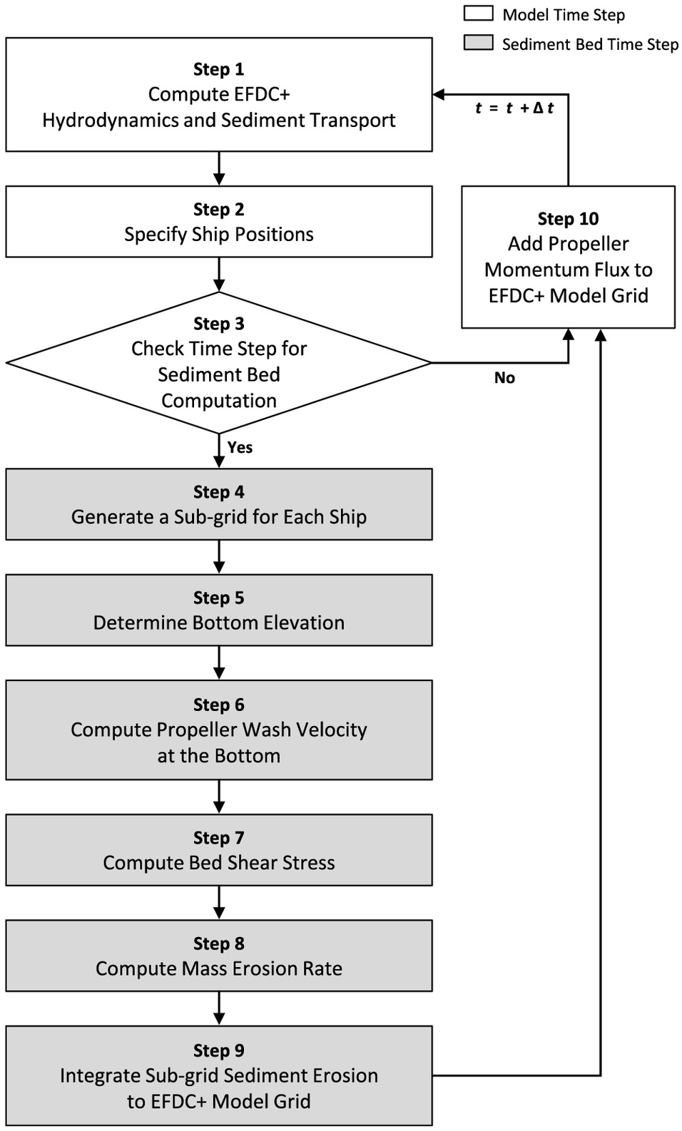

Step 1. Compute EFDC+ Hydrodynamics and Sediment Transport in the Water Column
For every EFDC+ model time step, a 3D hydrodynamic flow field is simulated at the model grid cell resolution, having a bottom elevation at each cell. The suspended sediment transport processes in the water column (i.e., advection, dispersion, and settling) are also computed in response to the hydrodynamic flow field. Fig. 3(a) displays an example of a two-dimensional (2D) plan view of the EFDC+ model grid cells. In this figure, the arrows indicate the depth-averaged ambient current velocity vectors simulated at a time step for each model cell.
Step 2. Specify Ship Positions
The location, heading, speed, applied power (expressed as propeller revolution speed or engine power), and depth to the propeller axis are specified for the ships to be modeled. These data can be derived from Automatic Identification System (AIS) data or other data sources.
Step 3. Check Time Step for Sediment Bed Computation
When the simulation time reaches the sediment bed time step, the computation will proceed to Step 4 for sediment resuspension implementation (i.e., interaction between the water column and sediment bed) with subgrids. Otherwise, the procedure will skip to Step 10 for calculation of the propeller-induced momentum in the hydrodynamic flow field based on model grid cells. The interval for the sediment bed computation is a user-defined model input parameter that can be equal to or greater than the model time step interval (DSI 2022).
Step 4. Generate Subgrid Points
Based on the specified ship positions, an independent 2D subgrid is generated behind each ship, as shown in Fig. 3(a). The subgrid will be used for calculating propeller wash–induced sediment resuspension mass in the following Steps 5 to 9.
Step 5. Determine Bottom Elevation
The bottom elevation of each subgrid point is determined by interpolating the bottom elevations of surrounding EFDC+ model grid cells. For the interpolation, an inverse distance squared scheme is applied to the distances between a subgrid point and model cell centers.
Step 6. Compute Propeller Wash Velocity at the Bottom
Given the subgrid bottom elevations and depth of the propeller, the bottom (i.e., water–sediment bed interface) velocities are computed. Fig. 4 presents the equations used in this algorithm to calculate the propeller wash velocity at the bottom for a specific location. The propeller wash formation characteristics and diffusion processes have been specified to differ explicitly among three regions: the efflux zone, the zone of flow establishment, and the zone of established flow.

The efflux zone indicates a short region behind the propeller () where the efflux velocity (i.e., the maximum propeller wash velocity occurring at the propeller face) does not decay (Hamill 1987), is the axial distance (m) from the propeller, and is the propeller diameter (m). In this study, the efflux velocity was calculated using either propeller revolution speed or ship engine power, depending on data availability. When propeller revolution speed is used, the efflux velocity (m/s) is computed following Fuehrer and Römisch (1977) as follows:where = propeller speed in revolutions per second (rps); and = propeller thrust coefficient (dimensionless). When ship engine power is used, the efflux velocity is determined using Maynord (2000) as follows:where = contracted propeller wash diameter (equivalent to 0.71 for a nonducted propeller and for a ducted propeller); and =water density (). The propeller thrust (N) is calculated as a function of applied engine power [horsepower (hp)] using the Toutant (1982) equation as follows:where = ship speed relative to the ground (). The efflux velocity magnitude is distributed approximately uniformly along the propeller plane within the efflux zone (Hamill 1987).
(1)
(2)
(3)
All subsequent propeller wash velocities beyond the efflux zone are dependent on the efflux velocity , as shown in Fig. 4. In the zone of flow establishment (), the propeller wash velocity decreases with distance as a result of lateral mixing, and the maximum velocity at an axial distance within this zone is computed following Hamill and Kee (2016). The lateral velocity profile within the zone of flow establishment forms two peaks due to the influence of the propeller hub, and the velocity at the longitudinal distance and the radial distance is calculated following Hamill (1987) and Berger et al. (1981). In the zone of established flow (), the propeller wash jet will dissipate into the background flow field and form only one maximum velocity peak at the propeller axis. The decay of the maximum axial velocity in this region is calculated using the empirical equation proposed by Hamill (1987), and the lateral profile of the velocity is defined according to Fuehrer and Römisch (1977).
Fig. 3(b) presents a vertical side view of the propeller wash velocity profiles, along with the subgrid points for velocity computation at the water–sediment bed interface. For ships with multiple propellers, the velocities are combined using the superposition principle. It should be noted that the propeller wash velocity computed at this step is used only for analytically calculating bed shear stress and sediment erosion mass at subgrid points, not for simulating the hydrodynamic flow velocities at the model grid cells.
Step 7. Compute Bed Shear Stress
Given the velocity at the bottom , a bed shear stress () for each subgrid point is computed using the Maynord (2000) approach as follows:where = vertical distance from the propeller axis to the sediment bed (m).
(4)
Step 8. Compute Mass Erosion Rate per Unit Area
Given the bed shear stress, an erosion rate is computed for each subgrid point using the sediment dynamics algorithms as developed by the Ziegler, Lick, and Jones (SEDZLJ) approach (Jones and Lick 2001; Thanh et al. 2008). When the bed shear stress () is greater than critical shear stress of the sediment bed (), the erosion rate () is calculated as follows:where and = data-based erosion rate constants (dimensionless) (Jones and Lick 2001; Thanh et al. 2008). The erosion rate is then converted to the mass erosion rate () as follows:where = sediment particle density (commonly ); and = total porosity of the sediment bed (dimensionless). In Fig. 3(c), the subgrid points with different levels of shading represent the resultant distribution of the propeller wash velocity at the bottom (from Step 6) or the bed shear stress (from Step 7) or the mass erosion rate (from Step 8).
(5)
(6)
Step 9. Integrate Subgrid Sediment Erosion to the EFDC+ Model Grid Cells
Given the erosion rate per unit area at each subgrid point (), the total mass erosion rate for each subgrid area () is calculated. In Fig. 3(d), the subgrid points and subgrid areas indicate the associated erosion quantities with different levels of shading.
Finally, the subgrid area erosion rates () are integrated into the EFDC+ model grid cells, denoted as (). Specifically, the eroded sediment mass () is allocated to the bottom water layer of the model cells (i.e., sediment resuspension). The resuspended sediments’ subsequent transport processes in the water column will then be simulated in response to the hydrodynamic flow field at the EFDC+ model grid resolution, as described in Step 1.
Step 10. Add Propeller Wash Momentum to EFDC+ Hydrodynamic Flow Field
For every model time step, using the ships’ positions and applied powers (rpm or hp) specified from Step 2, the momentum flux driven by the efflux velocity is added to the EFDC+ model cell where the ship’s propeller is located, as described subsequently.
Fig. 3(e) shows a conceptual diagram of the velocity vector components of a ship passing through a model grid cell in 2D plan view. Based on the angle between the ship’s heading and the cell rotation, the propeller efflux velocity [computed using Eqs. (1) or (2)] is split into the computational grid space in the and directions. Given the grid-oriented efflux velocity components , a specific momentum flux for each direction is computedwhere = propeller plane area (). The propeller momentum effect factor is a user-defined parameter (dimensionless) to account for momentum loss that is not directly simulated within the propeller location model cell. The value typically ranges between 0.3 and 0.7, according to observations from Kee et al. (2006) and Hamill and Kee (2016) that the actual cross-sectional area of the efflux velocity plane can be smaller than the propeller face area . Vertically, as shown in Fig. 3(f), the propeller wash–induced momentum fluxes and are distributed proportionately across the EFDC+ model grid water layers that the propeller intersects.
(7)
The propeller momentum flux will be added as a source term into the momentum equations of the EFDC+ hydrodynamic computation (Step 1) for the next model time step. The resulting flow field will then affect the subsequent movements of the resuspended sediments in the water column. EFDC+ uses a second-order accuracy discretization of numerical solutions for the momentum and transport equations. Specifically, in this development, horizontal kinetic turbulence is determined using the Smagorinsky model (Smagorinsky 1963), and vertical turbulence closure is solved using the Mellor and Yamada (1982) approach. In terms of numerical stability, the inclusion of the propeller wash momentum effect does not cause any critical numerical issues or instabilities in the hydrodynamic computation as long as the propeller parameters are appropriately specified using feasible data-based values (e.g., modeled propellers must be located vertically between the water surface and the sediment bed).
Repeat Propeller Wash Computation for Every Time Step
The aforementioned propeller wash computation processes will be repeated for every EFDC+ model time step where the ships are located within the model domain during the simulation.
Case Study
Tugboat Field Test at the San Diego Bay Naval Base
The method developed here was validated and tested using US Navy tugboat test events as a model application case. At a US Navy base in San Diego Bay, Wang et al. (2016) conducted a field study to observe propeller wash–induced velocity and bed erosion under controlled conditions using a tugboat Tractor C-14 on July 19, 2012. For this field survey, the tugboat was moored between Piers 4 and 5, with the bow pushing against a quay wall and the propellers thrusting toward the middle of the bay. During the low tide period (13:50 to 14:30), the propellers were operated at four different revolution speeds for different time periods. The propeller operation started with a period of 11 min at 20 rpm, which is the lowest rpm possible without stalling the tugboat engine. The revolution speed was then increased to 50 rpm for 11 min, followed by subsequent increases to 100 rpm for 9 min and 150 rpm for 9 min. After the 150-rpm period, the propellers were brought to a stop. An Acoustic Doppler Velocimeter (ADV) was installed at 110 m directly behind the tugboat to measure the water velocity at 15 cm above the bottom during the study period. Particle image velocimetry (PIV) was also deployed at the same location, and the PIV images were used to analyze the bottom elevation changes during the survey. Fig. 5 displays the locations of the ADV, PIV, and Tractor C-14.
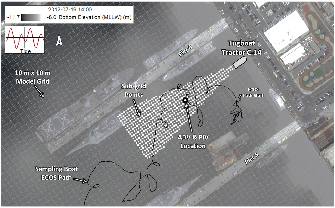
Wang et al. (2016) also investigated the concentrations of propeller wash resuspended sediments using Tractor C-14 at the same location on April 4, 2012. Once the tide was low (13:50 to 14:10), the tugboat engine power was increased consecutively to four different propeller speeds (20, 50, 100, and 150 rpm, each for 5 min) to generate a visible plume of resuspended sediments. After the tugboat engine stopped, a pump-sampling boat (named ECOS) tracked the tugboat-induced plume to collect water samples for about 1.5 h; the ECOS sampling boat’s path is shown in Fig. 5. The samples were pumped from between the surface and middepth of the water column; no sample was collected from bottom waters to prevent the sampling pump from inducing resuspension of bed materials. Total suspended sediments (TSS) concentrations and particle-size distributions were then analyzed in the laboratory from the samples collected during the field survey.
Model Development
This study developed a San Diego Bay tugboat test model using the algorithm presented in this paper and compared the simulated results with the field data to evaluate model performance. For model calibration, a model was built to simulate the field test for measurement of near-bed flow velocity and erosion depths (on July 19, 2012). All model parameters (e.g., hydrodynamics, sediment transport, and propeller wash) specified from the model calibration were then applied to the simulation of the sediment resuspension survey (on April 4, 2012) for model validation.
Fig. 5 displays the EFDC+ model grid cells, bottom elevations, and subgrid points for the tugboat Tractor C-14. The model domain used a horizontal grid of 4,556 cells with a uniform cell dimension of . A tide data time series from San Diego Bay station (ID 9410170) was applied to the open boundary cells of the model domain. Bottom elevations varied between and over the model domain. Due to the tides, water depth varied between 9 and 10 m around the tugboat test area during the simulation periods, and the model used 10 water layers for a vertical grid resolution. The model time step (i.e., hydrodynamic computation time step) was set to 0.2 s. Horizontal and vertical eddy viscosities were set to 0.003 and , respectively, to ensure the stability of the turbulence computation for ambient currents in the EFDC+ model grid cells.
The sediment bed conditions were defined uniformly over the model domain using a representative configuration. The critical shear stress of the sediment bed [ used for Eq. (5)] was set to because the initiation of sediment resuspension was observed when bed shear stress reached during the field program (Wang et al. 2016). The erosion rate constant was set to 1 because a linear relationship between shear stress and erosion rate was suggested for cohesive sediments (Kandiah and Arulanandan 1974; Wang et al. 2016). The erosion rate constant was calibrated based on the measured erosion depth data. Specifically, the bed shear stress and erosion depths observed over time from Wang et al. (2016) yielded an erosion rate constant ranging between 0.0001 and 0.0004 with respect to Eq. (5) when .
The sediment bed material composition was specified using two representative particle classes, consisting of 60% fine materials (clay + silt, 20-m uniform particle size with a settling speed of ) and 40% fine sand (180-μm uniform particle size with a settling speed of ) based on the field sample near Piers 4 and 5 collected by City of San Diego (2003). The total porosity of the sediment bed was set to 0.60 per Manger (1963), who reported the porosity of seafloor sediments with clay, silt, and fine sand in the San Diego Bay ranging between 0.51 and 0.74. The model used a time step of 1 s for the sediment bed computation.
For the propeller wash simulation, the model used the specifications of the tugboat Tractor C-14 provided by Wang et al. (2016). Table 1 summarizes the ship and propeller properties, propeller wash model parameters, and subgrid resolution used in this study (the sampling boat ECOS was not modeled). The tugboat Tractor C-14 had an installed engine power of 4,800 hp (1 horsepower is equivalent to 745.7 Watts), and twin-ducted propellers of 2.28 m diameter each were located at the bottom of the boat. The momentum effect factor was set to 0.5 (the middle of the typical value range of 0.3 to 0.7). A propeller wash subgrid was configured for tugboat Tractor C-14, which was a higher resolution than the model grid (i.e., ). The model simulated the tugboat operations with different propeller revolution speeds (20, 50, 100, and 150 rpm) for the field tests on July 19 (calibration run) and April 4 (validation run) as described by Wang et al. (2016).
| Property | Value |
|---|---|
| Ship length | 28.65 m |
| Ship beam | 10.36 m |
| Installed engine power | 4,800 hp |
| Propeller type | Twin ducted propellers |
| Number of propeller blades | 4 per propeller |
| Propeller diameter, | 2.28 m |
| Propeller hub diameter | 0.20 m |
| Distance between propellers | 4.88 m |
| Depth to propeller axis | 4.88 m |
| Propeller thrust coefficient, | 0.39 |
| Propeller blade area ratio, | 0.60 |
| Propeller pitch ratio, | 0.90 |
| Momentum effect factor, | 0.5 |
| Subgrid resolution | |
| Model grid resolution |
Note: 1 horsepower is equivalent to 745.7 Watts.
In addition to the rpm-based simulations, the model was also used to simulate the propeller wash at four different applied engine power (hp) levels (320, 800, 1,600, and 2,400 hp). The hp-based simulation was implemented by assuming that 50% of the installed engine power would be required for operating the propellers with a revolution speed of 150 rpm. This assumption was supported by the information in Wang et al. (2016) indicating that the low to medium propeller rotation speeds of Tractor C-14 were in the 20–150-rpm range. Additionally, the computed efflux velocity at 150 rpm [using Eq. (1)] is almost the same as the computed efflux velocity at 2,400 hp [using Eq. (2)], which is 50% of the installed engine power 4,800 hp (Table 1). The applied engine power for each of the four operation periods was then estimated with respect to the applied rpm levels relative to 150 rpm.
Results and Discussion
Flow Velocity at the Bottom
Fig. 6(a) compares the simulated flow velocities for the bottom water layer of the model grid cell at the ADV location with the measured data. The ADV raw data (gray dots) show flow velocities with large fluctuations due to turbulence, so this study considered the average and standard deviation of the fluctuating velocities for each rpm period. Open squares show the arithmetic averages of the measured data, and the whiskers represent ± one standard deviation in the measured data. Table 2 also presents the arithmetic averages of the ADV data, rpm-based model results, and hp-based model results for each period. Overall, the observed flow velocities increased with the propeller rotational speed, although the increase was not linear. For instance, when the propeller speed increased from 100 to 150 rpm (50% increase), the arithmetic average flow velocity only increased from 0.53 to (8% increase).

| Type | 20 rpm (320 hp) | 50 rpm (800 hp) | 100 rpm (1,600 hp) | 150 rpm (2,400 hp) | Stop |
|---|---|---|---|---|---|
| ADV data | 0.25 | 0.39 | 0.53 | 0.57 | 0.34 |
| Model (rpm) | 0.01 | 0.02 | 0.20 | 0.52 | 0.41 |
| Model (hp) | 0.14 | 0.28 | 0.44 | 0.56 | 0.40 |
The simulated propeller wash velocities increased with the applied rpms, shown as a bold line in Fig. 6(a). The flow velocities from the rpm-based model were almost zero during the 20-rpm period, but the underestimation diminished as the revolution speed increased. For the 150-rpm period, the simulated velocity magnitudes were very similar to the measured values. Compared with the rpm-based results, the hp-based simulation (dashed line) performed better in reproducing the ADV-measured velocities. The hp-based model results were all within one standard deviation of the arithmetic average of the measured data, although this model also underestimated the velocities for the low-propeller-speed periods. Additionally, the hp-based model simulated the velocity magnitudes as increasing nonlinearly with the applied engine power, which provides a better representation of the field data. The difference between the two model results originated from the different efflux velocity equations [Eqs. (1) and (2)] used for computing propeller momentum flux in the hydrodynamic simulations.
According to Wang et al. (2016), the underestimated flow velocities at low-propeller-speed conditions may be attributable to the tugboat driver’s uncertainty in propeller speed estimates during the test. In this case, the applied propeller revolution speeds were estimated and manually controlled by the tugboat driver, but the driver had difficulty maintaining the propeller speeds consistently without stalling the engine during the low-speed periods of 20 and 50 rpm. This information suggests that actual propeller rotating speeds could have been unsteady and inconsistent and could have been greater than the planned speeds, especially for the 20- and 50-rpm periods. The ADV flow velocity data showed the coefficient of variation (i.e., the ratio of the standard deviation to the average) for each speed period as 45% for 20 rpm, 40% for 50 rpm, 25% for 100 rpm, and 28% for 150 rpm. The greater coefficients of variation at the lower speed periods also support the idea that the uncertainty in propeller operation described previously could have significantly influenced the flow velocities measured during the 20- and 50-rpm periods.
Erosion Depth
Both the rpm-based and hp-based models were calibrated to reproduce the PIV-measured erosion depths. The calibrated erosion rate constants were 0.00027 for the rpm-based model and 0.00016 for the hp-based model, and both calibrated values were within the data-based range of 0.0001–0.0004. Fig. 6(b) compares the two model results and measured data for the cumulative erosion depths during the survey period. The measured PIV data indicated that erosion did not occur during the 20-rpm period; erosion started when the propeller speed was at 50 rpm. The erosion depth then increased continuously while the propellers were rotating, reaching 1.85 mm at 34 min. The measured erosion depth may contain an error of due to the pixel resolution of the PIV images (Wang et al. 2016). The sediment erosion rate (i.e., the slope of the curve) was notably higher at 150 rpm than during other periods. When the propellers were brought to a stop (after 36 min), the erosion depth decreased, indicating a bottom elevation increase as the sediments resuspended during the propeller operations settled back on the sediment bed.
Fig. 6(b) indicates that the hp-based model reproduced the measured erosion depths over the study period better than the rpm-based model did. The hp-based simulation presented the propeller wash–induced erosion starting at the 50 rpm (800 hp) period; the results then showed an erosion depth of 1.8 mm at 34 min, which is more consistent with the erosion behavior observed in the PIV data. For the rpm-based simulation, the propeller wash erosion did not occur until 18 min, likely due to the low flow velocities predicted for the 20- and 50-rpm periods. Consequently, to achieve the cumulative erosion depth of 1.8 mm at 34 min, the calibrated erosion rate constant for the rpm-based model was about 70% higher than the constant for the hp-based model. The temporal trend of erosion depths was adequately reproduced by both models, including the deposition of the resuspended sediment after the propellers were brought to a stop.
The Nash-Sutcliffe efficiency (NSE) coefficient was used to quantitatively evaluate the prediction performance of the rpm-based and hp-based models. The NSE coefficient can range from to 1, where an NSE of 1 indicates that the predictions reproduce the observed data perfectly and an NSE of 0 indicates that the predictions are as accurate as the data average value. The NSE value for the predicted erosion depths was 0.85 for the rpm-based simulation and 0.98 for the hp-based simulation, which suggests that both model results represented the measured data values well. Although the calibrated models exhibited a reasonable reproduction of both the measured flow velocities and erosion depths, it should be noted that the field data used for model evaluation in this study were only available at a location within the propeller wash zone. If data becomes available, further investigation would be necessary to verify the model performance in more extensive areas such as overlapping zones where both propeller wash and ambient flow are significant or outside of the propeller jet area.
Resuspended Sediment Concentration
For model validation, each of the rpm-based and hp-based models was used to simulate the sediment resuspension event of April 4, 2012. Table 3 compares the minimum, average, and maximum concentrations for TSS, fine materials (clay + silt), and fine sand in the water column from the field data and both model simulations. The field survey collected the resuspended sediment samples from surface to middepth water after the tugboat’s propellers stopped; the minimum of the measured TSS concentrations was . Accordingly, this study considered the model results from the top to middle water layers, which showed TSS concentrations equal to and greater than for the same period as the field data.
| Type | Total suspended sediments | Fines (clay + silt) | Sand | ||||||
|---|---|---|---|---|---|---|---|---|---|
| Minimum | Average | Maximum | Minimum | Average | Maximum | Minimum | Average | Maximum | |
| Data | 3.5 | 19.3 | 74.1 | 2.1 | 16.3 | 65.8 | 0.2 | 3.0 | 20.2 |
| Model (rpm) | 3.5 | 19.1 | 83.4 | 3.3 | 18.7 | 70.5 | 0.0 | 0.3 | 14.1 |
| Model (hp) | 3.5 | 15.7 | 72.5 | 3.1 | 15.4 | 59.6 | 0.0 | 0.3 | 15.4 |
Table 3 indicates that both models reproduced the overall measured data within for average concentrations and within for maximum concentrations. For TSS, the average concentration was predicted better by the rpm-based model, whereas the maximum concentration was reproduced better by the hp-based model. The higher TSS results from the rpm-based model compared with the hp-based model were understandable because the rpm-based model had the higher erosion rate constant , which would yield more sediment resuspension for the high-rpm periods (e.g., 100 and 150 rpm), as shown also in Fig. 6(b). The average concentration of fine materials was slightly better predicted by the hp-based model, whereas the two models showed about differences from the maximum concentration measured. For the fine sand–sized particles, both models underestimated the average data concentrations of .
Significant sources of uncertainty in the sample data must be noted when interpreting the validation results. First, the samples might not adequately have captured the representative plume structure because they were collected from different times and locations while the sampling boat was meandering in and around the propeller wash–induced sediment plume; the ship path is shown in Fig. 5. Specifically, inadequate vertical measurements and inadequate time averaging of samples would cause about 30% of uncertainty in the measured suspended sediment concentrations (Topping et al. 2011). In addition, the propeller wash from the sampling boat ECOS itself or other ship traffic nearby (not modeled in this study) could also have affected the movements of the resuspended sediments in the water column, disturbing the samples taken.
Fig. 7 compares the locations of TSS samples taken by ECOS and the horizontal extent of sediment plumes simulated by the models. In addition to the rpm-based and hp-based model results from validation runs that used a momentum effect factor of 0.5, this figure also contains the model results with the of 0, in which the simulations did not account for the propeller wash momentum effect to the flow field. In this figure, boundaries behind the tugboat indicate the region where the depth-averaged TSS concentrations of and greater occurred during each model simulation.
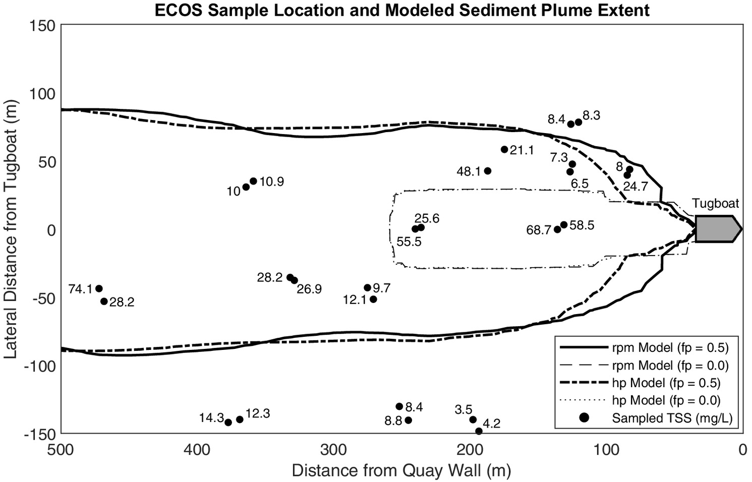
Overall, the model results are comparable between the rpm-based and hp-based runs, but the results are notably different between and . From the models with , the resuspended sediments were transported over a larger area in longitudinal and lateral directions, indicating more active advection and dispersion in the water column due to the increased flow energy from the propeller momentum. The horizontal extent of the simulated sediment plumes covered most of the locations where the ECOS observed the sediment plume. In contrast, the models with showed that the resuspended sediments remained in the area closer to where they were eroded, due to the small ambient flows in the model domain. Consequently, the simulated sediment plume area with exhibited a much smaller area than the ECOS measurement extent.
A tidal current propagating from north to south also influenced the plume distribution; this resulted in the low TSS concentrations observed in the south (outside the modeled plume in Fig. 7) 1 h and longer after the propeller stopped. Although the model applied the tide measurement data to the model domain boundaries, the tidal currents were underpredicted because the model domain extent () was not sufficiently large. Despite this limitation, the validation results suggest that both rpm-based and hp-based models with propeller momentum effects could reasonably reproduce the sediment plume area observed from the event of April 4, 2012.
Vertical Profiles of TSS Concentrations
This study also examined the vertical profiles of resuspended sediment concentrations in the water column from the model calibration runs that simulated the field test on July 19, 2012. In general, sediment resuspension yields the maximum TSS concentration near the bottom, and the concentration decreases toward the water surface. Because the field data did not provide the vertical distributions of resuspended sediments, this study assumed analytical TSS profiles from the Hong et al. (2016) approach to be the field observations and compared them with the model results. From flume experiments, Hong et al. (2016) proposed an empirical equation for the vertical profiles of propeller wash–induced suspended sediment concentrations by adopting the Rouse (1938) formulawhere = sediment concentration at a distance above the sediment bed; = concentration at a reference level (i.e., equilibrium near-bed sediment concentration) where is usually considered as 5% of water depth ; and = Rouse number that specifies the slope of the vertical concentration profile in the water column. The constant Rouse number was proposed to be valid for the zone beyond behind the propeller, in which a densimetric Froude number is between 7.49 and 31.49 (Hong et al. 2016).
(8)
Fig. 8 compares the vertical TSS profiles from the Hong et al. (2016) method with the model results at 110 m behind the tugboat from the 150-rpm period of the rpm-based simulation [Fig. 8(a)] and from the 2,400-hp period of the hp-based simulation [Fig. 8(b)]. The location considered () and its densimetric Froude number calculated from the ADV data () are within the valid range for using the Hong et al. (2016) method. In this figure, bold lines represent the predictions from the model calibration runs that used a momentum effect factor of 0.5. To demonstrate how the variation of impacts the model results, this figure also includes the concentration profiles from the simulations with values of 0.7 and 0.3, which are the upper and lower bounds of the typical range, respectively. Additionally, the model results are shown for , indicating no propeller wash momentum effect.

Overall, the model with (i.e., the calibration model) and the Hong et al. (2016) empirical approach provided similar vertical profiles, decreasing TSS concentrations gradually from the bottom to top, which indicates that the vertical mixing of resuspended sediments due to propeller wash is comparable. By applying the profiles from the Hong et al. (2016) approach to be the field observations, the model results with yielded NSE values of 0.97 for both rpm-based and hp-based runs, showing better performance than the other factors used, as presented in Table 4. Whereas the model with showed overestimation (i.e., more mixing) and the model with showed underestimation (i.e., less mixing), their NSE values of 0.87–0.95 indicated a reasonable reproduction of the Hong et al. (2016) empirical profiles. In contrast, the model with exhibited high TSS concentrations only near the bottom, which is not comparable with Hong et al.’s (2016) results (i.e., negative NSE). In this case, the simulated flow field represented the quiescent tidal condition without propeller wash–induced flow velocities, so the resuspended sediments were not mixed vertically and stayed near the bottom during the simulation. These results support the conclusion that the propeller wash models developed here (e.g., ) could reasonably reproduce the vertical profiles of resuspended sediment concentrations in the water column by accounting for the propeller momentum–induced hydrodynamic flow field.
| Type | Propeller momentum factor, | |||
|---|---|---|---|---|
| 0.7 | 0.5 | 0.3 | 0.0 | |
| Model (rpm) | 0.88 | 0.97 | 0.95 | |
| Model (hp) | 0.87 | 0.97 | 0.93 | |
Sensitivity of Erosion Depth and Deposition Area
This study also investigated the sensitivity of model results for maximum erosion depth and area of resuspended sediments deposited by varying model input elements of the San Diego Bay case, as shown in Fig. 9. For this analysis, the calibration runs (July 19, 2012) of rpm-based and hp-based models were selected as the base simulations. Six levels of percentage change (, , , , , and ) were applied to each of model inputs, including the depth to propeller axis (4.88 m), propeller momentum effect factor (), a series of propeller revolution speeds (20, 50, 100, and 150 rpm) were used in the rpm-based model, and a series of applied engine powers (320, 800, 1,600, and 2,400 hp) were used in the hp-based model. A total of 36 model runs were simulated until 2 h after the tugboat engine stopped, allowing most of the resuspended sediments to settle. In Fig. 9, the -axis indicates the percentage of model result changes compared with the base simulation results. For the model outputs, the maximum erosion depth following the 2-h runs was considered, and the length and width of the deposition area were determined based on the area where the mass of resuspended sediments deposited was greater than .

For the maximum erosion depth, both rpm-based and hp-based simulations were most sensitive to the changes in the depth to the propeller axis (circle marker). As the propeller axis goes deeper into the water, the propellers get closer to the seabed, leading to more sediment erosion due to the increased propeller wash impacts. The simulated maximum scour also increased when either the propeller revolution speed (asterisk marker) or the applied engine power (cross marker) increased. The propeller speeds in the rpm-based runs yielded more impacts on the erosion depth results than the applied engine powers in the hp-based runs. Such sensitivity differences are derived from the different efflux velocity equations [Eqs. (1) and (2)], which are used for computing all subsequent propeller wash velocities and erosion rates at subgrid points in the models (Steps 6–8). The propeller momentum effect factor (triangle marker) showed the least influence on the maximum erosion depth because this parameter only affects the flow field computation at the EFDC+ model grid cells (Step 10), not the erosion rate computation at the propeller wash subgrid points.
For the length of the resuspended sediment deposition area, the propeller momentum effect factor showed notable impacts on the model results. With a higher momentum effect factor, the resuspended sediments were transported over a larger area due to the increased flow energy from the propeller momentum, resulting in the deposition mass being significantly dispersed in longitudinal and lateral directions. In contrast, the model with a lower momentum effect factor showed a smaller deposition area; the resuspended sediments were deposited closer to where they were eroded earlier due to the low energy in the flow field. The length of the resuspended sediment deposition area also increased as the propeller revolution speed or the applied engine power increased; these model inputs affect the bed erosion calculation (Steps 6–8) and flow field computation (Step 10). The depths to the propeller axis also exhibited a positive correlation with the length of the deposition area but showed smaller impacts than the other input elements.
Although displaying less variation than in the other cases mentioned previously, the width of the resuspended sediment deposition area increased when the three considered model inputs increased. In both rpm-based and hp-based simulations, the depth to the propeller axis and momentum effect factor showed comparable impacts on the lateral dispersion of the resuspended sediments. The propeller revolution speeds and applied engine power exhibited more influence than the other inputs because they increased both the erosion rate (Steps 6–8) and flow energy (Step 10) during the simulations. The findings from this investigation not only help identify the impacts of model input elements on the results but also demonstrate that the propeller wash models developed here predict sediment resuspension and redistribution consistent with the model theory of physical processes.
Assessment of Model Grid Resolution
Model result analysis included an evaluation of the model grid to ensure it was appropriately defined for the resolution of the problem. In this study, the calibrated model results (i.e., grid) were compared with simulations with various model grid resolutions to assess whether the calibration model grid was fine enough to address the propeller wash impacts on the hydrodynamic and sediment transport processes considered. For this analysis, the calibration case was modeled using three uniform grid resolutions: 5 × 5, 20 × 20, and . In all cases, the models used a subgrid resolution of , except that a subgrid resolution was used for the 5-m grid model to ensure that each model cell contained at least four subgrid points. These grid test models used the same general parameters and inputs as specified for the 10-m grid calibration model. However, Tractor C-14’s two propellers, each having a diameter of 2.28 m with a 4.88-m distance between the propellers (Table 1), stretched over two model cells in the 5-m grid, whereas the propellers were located within a single cell for the coarser grids. Thus, in the 5-m grid model, the momentum flux driven by the two propellers was evenly distributed between the two model cells where the propellers were located (i.e., a 50% fraction each).
Fig. 10(a) displays the simulated flow velocities from the hp-based models with various grid resolutions for the bottom water layer of the model cell at the ADV location. Overall, the 5-m grid model and the 10-m grid model exhibited comparable flow velocities driven by the propeller wash momentum flux, with a correlation coefficient of 0.99. Moreover, both models successfully reproduced the measured velocity magnitudes at the 2,400-hp period, and their results were all within one standard deviation of the data average for each period. On the other hand, the coarser grid models (e.g., 20- and 30-m grids) significantly underestimated the velocity magnitudes. Lower flow velocities were simulated as the grid resolution decreased, indicating that the propeller momentum–induced velocities were averaged over too large of an area. These results indicate that the 10-m grid is sufficiently fine enough to represent the propeller wash jet characteristics at the ADV location, similar to the 5-m grid.

Fig. 10(b) presents the simulated erosion depths from the various grid model runs for the model cell at the PIV location. Similar to the flow velocity results, the 5-m grid model and the 10-m grid model resulted in almost identical erosion depths during the simulations. The 2.25-m subgrid points within the 5-m grid model cell and the 4.5-m subgrid points within the 10-m grid model cell yielded almost the same erosion rates (cm/s) induced by the propeller wash. Specifically, both models exhibited an erosion depth of 1.8 mm at 34 min, close to the measured value of 1.85 mm.
In contrast, erosion depths were notably underestimated by the coarser grid models due to the large cell areas at the PIV location containing too many subgrid points with lower erosion rates. Consequently, the 20- and 30-m grids yielded erosion depths at 34 min of 1.50 and 1.07 mm, respectively. The findings from this assessment suggest that both the model grid and subgrid resolutions of the calibration model were fine enough to represent the observed propeller wash effects for the hydrodynamic and sediment transport behaviors considered in this study.
Model Uncertainty Discussion
The numerical model results presented in this paper inherently contain uncertainty. Sources of model uncertainty are commonly classified into three categories (Ajami et al. 2007): the mathematical structure of the modeling method, model input data, and model parameter values. Each uncertainty type identified in this modeling study is briefly discussed.
First, the developed numerical method applies several simplifications and assumptions to implement the propeller wash processes using mathematical equations. Specifically, the propeller wash velocity equations used in the model algorithm were empirically derived from laboratory and field experiments under certain conditions, so the simulation results will change if other formulas are used for the velocity computation. For instance, in this study, the rpm-based simulation [using Eq. (1)] and the hp-based simulation [using Eq. (2)] provided different flow velocity and sediment transport results throughout the model validation and sensitivity tests.
Second, the data used for the model inputs could be subject to the uncertainty associated with measurement errors or data limitations, which might produce inaccurate predictions even if a suitable modeling method is used. This study noted that underestimated flow velocities at low-propeller-speed conditions could result from uncertainty in propeller speeds not well controlled by the tugboat driver. The engine power (hp) levels estimated using propeller speeds (rpm) for hp-based simulations may also contain significant uncertainty. Additionally, this study used a homogeneous sediment bed configuration for the model conditions due to limited sediment data availability. Specifically, the particle-size distribution at the test site was not documented by Wang et al. (2016), so the sediment bed condition was modeled using two representative size classes based on the City of San Diego (2003). Such uncertainty in the sediment bed may have contributed to the models underestimating (or overestimating) the measured concentrations for resuspended sediments.
Third, any uncertainties in the values assigned to the model parameters, which were difficult to measure directly, could also result in uncertainty in the model predictions. In this study, the model validation and sensitivity analysis demonstrated the impacts of the momentum effect factor on the simulation results for resuspended sediment concentrations, erosion depth, and deposition area induced by propeller wash. Additionally, eddy viscosity values for hydrodynamics and erosion rate parameters for sediment beds could also be subject to uncertainty because they were specified or calibrated based on the model conditions.
Conclusion
This study presented a numerical modeling approach to simulate sediment resuspension and transport processes with a fully coupled representation of hydrodynamics, sediment transport, and propeller wash from ship traffic. The propeller wash–induced sediment resuspension was calculated based on an independent subgrid and then integrated into the model grid. The propeller wash momentum flux was directly incorporated into the model grid for flow field computation, and the resulting flow field was used for computing the subsequent movement of the resuspended sediments. The methodology was able to dynamically simulate the combination of propeller wash–induced processes, including scour, sediment resuspension, subsequent movements of the resuspended sediments in the water column, and deposition of the resuspended sediments on the sediment bed.
For the case study using the San Diego Bay tugboat test events (Wang et al. 2016), two models were developed to simulate the propeller wash, based on propeller revolution speed (rpm-based model) and tugboat engine power (hp-based model). Each model was calibrated using ADV-measured flow velocities and PIV-measured erosion depths. The hp-based model predicted the flow velocities to increase nonlinearly with the applied engine power, which provided a better representation of the field data than the rpm-based model; the hp-based model results were all within one standard deviation of the measured field data average. Both the rpm-based and hp-based models adequately reproduced the temporal trend of measured erosion depths with a NSE value of 0.85 and 0.98, respectively.
From the model validation, the two models predicted the measured concentrations for TSS, fine materials (clay + silt), and sand in the water column within for arithmetic average concentrations and within for maximum concentrations. The horizontal extent of the sediment plumes simulated from the validation models were comparable to the ECOS-measured plume locations. The model results provided vertical profiles of TSS concentrations similar to predictions by the Hong et al. (2016) approach, with concentrations decreasing gradually from the bottom to surface, which accounts for the vertical mixing of resuspended sediments due to propeller wash velocities. Overall, simulating the increased flow energy from propeller momentum, resulting in more active advection and dispersion in the water column, reproduced the horizontal and vertical distributions of resuspended sediments better than simulating only ambient currents. Furthermore, the sensitivity test also indicated that the increased flow energy from propeller momentum yielded substantial advection and dispersion of resuspended sediments. Additionally, the simulated maximum scour induced by propeller wash is significantly dependent on the propeller rotational speed, the applied ship engine power, and the distance between the propellers and the sediment bed.
This paper noted the uncertainties associated with the limited field data on hand when discussing simulation results. Such uncertainties can be addressed if adequate field data under well-controlled conditions become available, allowing a better understanding of propeller wash behaviors. Additionally, quantitative assessment of uncertainty in model predictions can be achieved by a formal, comprehensive analysis with Bayesian inference methods (Kuczera et al. 2006; Jung et al. 2018).
Several notable avenues are also available for future research, as follows. First, consideration should be given to modeling the propeller wash–induced bed load process, which will be significant at sites with noncohesive sediments. Second, the bottom friction coefficient used for the propeller wash–induced shear stress calculation [Eq. (4)] can be dependent on sediment bed roughness as the combination of skin friction and form drag. Third, the actual flow field around a moving ship would be more complicated than the analytical velocity profiles used in this study. Specifically, significant turbulent wakes can occur when a ship’s main body moves through the water, and propeller wash from cycloidal propulsion systems could result in more complex jet profiles. Addressing these components would benefit follow-up studies by enhancing the applicability of the modeling framework presented here.
Data Availability Statement
Some or all data, models, or code generated or used during the study are available in a repository or online in accordance with funder data retention policies. EFDC+ source codes, including the propeller wash features presented in this study, are fully open-source and available online (https://github.com/dsi-llc/EFDCPlus).
Acknowledgments
This research was financially supported by ExxonMobil Environmental and Property Solutions Company, and we appreciate the support of Frank Messina. The authors also thank Dr. Doug Blue and Stacy Hall de Gomez for their reviews of this article.
References
Ajami, N. K., Q. Duan, and S. Sorooshian. 2007. “An integrated hydrologic bayesian multimodel combination framework: Confronting input, parameter, and model structural uncertainty in hydrologic prediction.” Water Resour. Res. 43 (1): W01403. https://doi.org/10.1029/2005WR004745.
Berger, W., K. Felkel, M. Hager, H. Oebius, and E. Schale. 1981. “Courant provoque par les bateaux protection des berges et solution pour eviter l’erosion du lit du haut rhin.” In Proc., 25th Int. Navigation Congress. Edinburgh, Scotland: PIANC.
City of San Diego. 2003. “An ecological assessment of San Diego Bay: A component of the Bight’98 regional survey.” In City of San Diego ocean monitoring program. San Diego: Dept. of Metropolitan Wastewater, Environmental Monitoring and Technical Services Division.
Clarke, D., K. J. Reine, C. Dickerson, C. Alcoba, J. Gallo, B. Wisemiller, and S. Zappala. 2015. Sediment resuspension by ship traffic in Newark Bay, New Jersey. Vicksburg, MS: USACE, Engineer Research and Development Center.
DSI. 2022. “EFDC+ theory document version 10.3.” Accessed May 5, 2022. https://www.eemodelingsystem.com/wp-content/Download/Documentation/EFDC_Theory_Document_Ver_10.3_2022.05.03.pdf.
Fuehrer, M., and K. Römisch. 1977. “Effects of modern ship traffic on inland and ocean waterways.” In Proc., 24th Int. Navigation Congress, 236–244. Leningrad, Russia: PIANC.
Hamill, G. A. 1987. “Characteristics of the screw wash of a manoeuvring ship and the resulting bed scour.” Ph.D. thesis, Dept. of Civil Engineering, Queen’s Univ. of Belfast.
Hamill, G. A., and C. Kee. 2016. “Predicting axial velocity profiles within a diffusing marine propeller jet.” Ocean Eng. 124 (Sep): 104–112. https://doi.org/10.1016/j.oceaneng.2016.07.061.
Hammack, E. A., D. S. Smith, and R. L. Stockstill. 2008. Modeling vessel-generated currents and bed shear stresses. Vicksburg, MS: USACE, Engineer Research and Development Center.
Hamrick, J. M. 1992. A three-dimensional environmental fluid dynamics computer code: Theoretical and computational aspects. Gloucester Point, VA: Virginia Institute of Marine Science, College of William and Mary.
Hayter, E., P. Schroeder, N. Rogers, S. Bailey, M. Channell, and L. Lin. 2016. Evaluation of the San Jacinto Waste Pits feasibility study remediation alternatives. ERDC Letter Report. Vicksburg, MS: USACE, Engineer Research and Development Center.
Hong, J. H., Y. M. Chiew, S. C. Hsieh, N. S. Cheng, and P. H. Yeh. 2016. “Propeller jet–induced suspended-sediment concentration.” J. Hydraul. Eng. 142 (4): 04015064. https://doi.org/10.1061/(ASCE)HY.1943-7900.0001103.
Jones, C. A., and W. Lick. 2001. SEDZLJ: A sediment transport model. Final Report. Santa Barbara, CA: Univ. of California.
Jung, J. Y., J. D. Niemann, and B. P. Greimann. 2018. “Combining predictions and assessing uncertainty from sediment transport equations using multivariate Bayesian model averaging.” J. Hydraul. Eng. 144 (4): 04018008. https://doi.org/10.1061/(ASCE)HY.1943-7900.0001436.
Kandiah, A., and K. Arulanandan. 1974. “Hydraulic erosion of cohesive soils.” Transp. Res. Rec. 497 (Dec): 60–68.
Kee, C., G. A. Hamill, W. H. Lam, and P. W. Wilson. 2006. “Investigation of the velocity distributions within a ship’s propeller wash.” In Proc., 16th Int. Offshore and Polar Engineering Conf., 451–456. Cupertino, CA: International Society of Offshore and Polar Engineers.
Kuczera, G., D. Kavetski, S. Franks, and M. Thyer. 2006. “Towards a bayesian total error analysis of conceptual rainfall-runoff models: Characterising model error using storm dependent parameters.” J. Hydrol. 331 (1): 161–177. https://doi.org/10.1016/j.jhydrol.2006.05.010.
Manger, G. E. 1963. Porosity and bulk density of sedimentary rocks. Washington, DC: US Atomic Energy Commission.
Mateus, S. V., F. A. Bombardelli, and S. G. Schladow. 2020. “Boat induced sediment resuspension and water clarity in shallow flows.” In River flow 2020, 1333–1341. London: CRC Press.
Maynord, S. T. 2000. Interim report for the Upper Mississippi River— Illinois waterway system navigation study: Physical forces near commercial tows. Vicksburg, MS: USACE, Engineer Research and Development Center.
Mellor, G. L., and T. Yamada. 1982. “Development of a turbulence closure model for geophysical fluid problems.” Rev. Geophys. 20 (4): 851–875. https://doi.org/10.1029/RG020i004p00851.
Michelsen, T. C., C. D. Boatman, D. Norton, C. C. Ebbesmeyer, and M. D. Francisco. 1998. “Transport of contaminants along the Seattle waterfront: Effects of vessel traffic and waterfront construction activities.” Water Sci. Technol. 37 (6): 9–15. https://doi.org/10.2166/wst.1998.0729.
Poon, Y. D., A. Luke, S. Ueoka, A. Jirik, and J. Vernon. 2016. “Contaminated sediment transport in the Greater Los Angeles and Long Beach Harbor: Incorporating propeller-induced re-suspension of sediment.” In World environmental and water resources congress 2016. West Palm Beach, FL: ASCE.
Romberg, G. P. 2005. “Recontamination sources at three sediment caps in Seattle.” In Proc., 2005 Puget Sound Georgia Basin Research Conf., 236–244. Seattle: Puget Sound Institute.
Rouse, H. 1938. “Experiments on the mechanics of sediment suspension.” In Proc., 5th Int. Congress for Applied Mechanics. New York: John Wiley & Sons.
Smagorinsky, J. 1963. “General circulation experiments with the primitive equations: I. The basic experiment.” Mon. Weather Rev. 91 (3): 99–164. https://doi.org/10.1175/1520-0493(1963)091%3C0099:GCEWTP%3E2.3.CO;2.
Thanh, P. H. X., M. D. Grace, and S. C. James. 2008. Sandia national laboratories environmental fluid dynamics code: Sediment transport user manual. Livermore, CA: Sandia National Laboratories.
Topping, D. J., D. M. Rubin, S. A. Wright, and T. S. Melis. 2011. Field evaluation of the error arising from inadequate time averaging in the standard use of depth-integrating suspended-sediment samplers. Reston, VA: US Geological Survey.
Toutant, W. T. 1982. “Mathematical performance models for river tows.” In Great Lakes and great rivers section. Clarksville, IN: Society of Naval Architects and Marine Engineers.
Trim, H. 2004. Restoring our river; protecting our investment: Duwamish River pollution source control. Review report. Seattle: Duwamish River Cleanup Coalition.
Wang, P. F., I. D. Rivera-Duarte, K. Richter, Q. Liao, K. Farley, H. C. Chen, J. Germano, K. Markillie, and J. Gailani. 2016. Evaluation of resuspension from propeller wash in DoD harbors. ESTCP ER-201031. San Diego: Space and Naval Warfare Systems Center.
Ziegler, K., D. Nangju, and F. Chen. 2019. “Development and application of propwash resuspension model for Newtown Creek.” In Proc., Int. Conf. on the Remediation and Management of Contaminated Sediments. Columbus, OH: Battelle.
Information & Authors
Information
Published In

Journal of Hydraulic Engineering
Volume 149 • Issue 5 • May 2023
Copyright
This work is made available under the terms of the Creative Commons Attribution 4.0 International license, https://creativecommons.org/licenses/by/4.0/.
History
Received: Feb 1, 2022
Accepted: Dec 12, 2022
Published online: Mar 10, 2023
Published in print: May 1, 2023
Discussion open until: Aug 10, 2023
ASCE Technical Topics:
- Coasts, oceans, ports, and waterways engineering
- Computer models
- Engineering fundamentals
- Fluid dynamics
- Fluid mechanics
- Hydrodynamics
- Hydrologic engineering
- Infrastructure
- Models (by type)
- Numerical models
- River engineering
- Sediment
- Sediment transport
- Ships
- Traffic models
- Transportation engineering
- Water and water resources
- Water transportation
Authors
Metrics & Citations
Metrics
Citations
Download citation
If you have the appropriate software installed, you can download article citation data to the citation manager of your choice. Simply select your manager software from the list below and click Download.
Cited by
- Channel Sedimentation Processes, Navigation Channel Sedimentation Solutions, 10.1061/9780784485149.ch2, (13-30), (2023).