Improving Flood Inundation Mapping Accuracy Using HEC-RAS Modeling: A Case Study of the Neches River Tidal Floodplain in Texas

Qian, Qin; Edwards, Darius J.; Zhang, Yu; Haselbach, Liv

doi:10.1061/JHYEFF.HEENG-6037

Open access

Case Studies

Apr 24, 2024

Improving Flood Inundation Mapping Accuracy Using HEC-RAS Modeling: A Case Study of the Neches River Tidal Floodplain in Texas

Authors: Qin Qian, M.ASCE https://orcid.org/0000-0002-3992-9082 [email protected], Darius J. Edwards [email protected], Yu Zhang [email protected], and Liv Haselbach, F.ASCE https://orcid.org/0000-0001-6256-9890 [email protected]Author Affiliations

Publication: Journal of Hydrologic Engineering

Volume 29, Issue 4

https://doi.org/10.1061/JHYEFF.HEENG-6037

PDF

Abstract

The Neches River Tidal floodplain has been historically prone to flooding, resulting in critical shutdowns of refineries and port transit. This study implements a one-dimensional (1D) and a coupled 1D/two-dimensional (2D) Hydrological Engineering Center’s River Analysis System (HEC-RAS) model including the bathymetry data of the main channel to develop flood inundation maps under different hydrological and hydraulic conditions. Comparing the 1D model with the FEMA Base Level Engineering (BLE) model, the results show that flood inundation maps are highly sensitive to the bathymetry data, which is essential to simulate accurate flood inundation maps for a river with dredged waterways. The inundation maps simulated by the 1D/2D model have better agreement with the high-water marks than the 1D model during Hurricane Harvey. In conclusion, coupled 1D/2D modeling provides a more realistic depiction of flood threats with the limited available data and is superior to the FEMA BLE model for producing accurate flood inundation maps of the Neches River Tidal floodplain.

Introduction

Recently, catastrophic flooding events have been recorded all over the world (Blöschl et al. 2017) and are expected to increase in frequency and intensity under changing climate conditions in the United States (Kossin 2018; Blake and Zelinsky 2018). The southeast Texas Gulf coastal region experienced historical flooding that caused both fatalities and significant damage during Hurricane Harvey in 2017 (NOAA 2017) and Tropical Storm Imelda in 2019 (NOAA 2019). The Neches River Tidal floodplain has been historically prone to major riverine and storm surge flooding events (Maymandi et al. 2022; Lee 2022) and an increasing incidence of nuisance flooding produced by localized storms (Qian et al. 2022; Haselbach et al. 2023). Part of the Neches River Tidal section functions as a dredged waterway running between the Port of Beaumont to Sabine Lake, where heavy petrochemical refineries are situated along the west side of the ship channel. The Port of Beaumont was responsible for $12.6 billion in gross domestic product and $18.8 billion in direct international trade value in 2018 (Hegar 2018). Flood inundation has resulted in critical shutdowns of oil-refining facilities and port transit, interrupting the supply chain of oil and goods for the region and nation (Blake and Zelinsky 2018). It is known that the implementation of flood mitigation measures, assessment of flood vulnerability, comparative risk analysis, and risk mapping are major flood damage reduction approaches (Merz et al. 2010). Flood inundation mapping is an important step in developing effective flood damage assessment for evaluating flood potential, making investment decisions, and creating flood policies (Buchele et al. 2006; Weaver 2016; Mihu-Pintilie et al. 2019; Song et al. 2019; Ghimire and Sharma 2020). The FEMA Base Level Engineering (BLE) floodplain analysis of the Neches River basin (FEMA 2019) provided floodplain inundation maps for 10-year, 25-year, 50-year, 100 minus-year, 100-year, 100 plus-year, and 500-year flood events (Asquith and Roussel 2009) using 10-m digital elevation model (DEM) data obtained from the United States Geological Survey (USGS) National Map database (USGS 2019). Local stakeholders and agencies have adopted FEMA BLE inundation maps and taken into consideration high-water marks from Hurricane Harvey for local recovery. Depending on the types of infrastructures, different design judgements, for example, above 0.10 m (4 in.), 0.15 m (6 in.), 0.30 m (1 foot), or at the same high-water marks of Hurricane Harvey, were considered for rebuilding houses, drainage systems, pump stations, highways, industry facilities, and so on (personal communication with city engineers, county engineers, drainage district managers and engineers, and district engineers of Texas Department of Transportation). No flood inundation map is available for extreme flood events caused by hurricanes or tropical storms. Therefore, there is an urgent need to have predictive capabilities of flood inundation maps for mitigating impacts and assisting in recovery efforts of the Neches River Tidal floodplain.

Selecting an appropriate flood inundation model for stakeholders to restore the floodplain and mitigate flood damage is challenging because model simulations are sensitive to hydrological and hydraulic analysis, including other socioeconomic factors (Ghimire and Sharma 2020). With the advent of efficient numerical methods in combination with high-performance computing resources, various flood inundation models have been developed to support these decision-making processes (Enea et al. 2018; Mihu-Pintilie et al. 2019; Hutanu et al. 2020; Saksena et al. 2020; Garcia et al. 2020; Ghimire and Sharma 2020). The simplest one-dimensional (1D) models are computationally efficient along river channels (Wang and Zhang 2019; Kastali et al. 2021) but are subject to the inability to simulate flood wave diffusion. Two-dimensional (2D) models simulate the floodplain flow to demonstrate the extent of floods and overcome 1D limitations to improve uncertainty (Teng et al. 2017; Sharma and Regonda 2021). Two-dimensional models are recommended in cases when the water is expected to overtop levees and the flow direction may change, spreading across a large area (Kadir et al. 2019; Hankin et al. 2019). Several flood inundation mapping models using the 2D Hydrologic Engineering Center’s River Analysis System (HEC-RAS) (Brunner 2016, 2021) have also been developed, for example, the Lower Region of Brazos River Watershed in Texas (Bhandari et al. 2017), Prayagraj at the confluence of River Ganga and Yamunain in India (Kumar et al. 2002), rivers in Kazakhstan (Ongdas et al. 2020), the lower region of Purna Basin (Pathan and Agnihotri 2020), and the coastal plain of Virginia (Morsy et al. 2021). The 2D HEC-RAS model has been applied for hydrological, hydraulic, and reservoir operations to assess flood impacts during Hurricane Harvey in West Harris County, Texas (Garcia et al. 2020), and to improve urban flood hazard maps with the flood mitigation capacity of reservoirs in Bacau City, Romania (Mihu-Pintilie et al. 2019). Because the 2D HEC-RAS model is computationally complex, a coupled 1D/2D HEC-RAS approach allows users to model 1D in the main channel and 2D computational meshes in the floodplain to simulate flood inundation with less computational time while improving the model accuracy. The coupled 1D/2D HEC-RAS has simulated flood inundation in Surat city (Patel et al. 2017), a coastal urban area combining sea-level rising and extreme flood events (Pasquier et al. 2019), and the 2002 Baeksan levee failure event on the Nam River in South Korea (Dasallas et al. 2019).

To provide a more realistic perspective for local recovery and rebuilding, the objective of this study was to develop 1D and coupled 1D/2D HEC-RAS (version 5.0.7) models to improve flood inundation mapping accuracy for design and extreme flood events for decision makers to take into consideration when making decisions on mitigating flood impacts of the Neches River Tidal floodplain and to enhance local resiliency. Both models were established based on a light detection and ranging (LiDAR)–derived DEM and processed with the geographical information system (GIS) ArcMap 10.7.1 (ESRI 2019). The 1D HEC-RAS model was developed from the FEMA BLE floodplain analysis of the Neches River basin (FEMA 2019) and updated with the bathymetry data provided by the US Army Corps of Engineers (USACE personal communication). The coupled 1D/2D HEC-RAS model was developed to investigate the accuracy of large-scale flood inundation maps. Streamflow hydrographs at USGS Gage Station 08041780 were applied to calibrate and validate the 1D channel Manning’s roughness coefficients. The recorded USGS high-water marks for Hurricane Harvey were applied to calibrate roughness coefficients in the 2D area and weir coefficients along the channel for the coupled 1D/2D model. Finally, the coupled 1D/2D model was applied to simulate the flood inundation maps for design and extreme flooding events to assess flood vulnerability and inform vulnerability and investment decisions on flood reduction measures.

Study Area and Data

The study area is located within the Neches River Tidal watershed, as shown in Fig. 1(a), which is composed of parts of Jefferson and Orange counties in southeast Texas, including the cities of Port Arthur, Beaumont, Port Neches, Bridge City, Rose City, Vidor, and Pine Forest. A total of about 550 square kilometers (212 square miles) of drainage area consists of low, flat plains, with some of the area being tidal marshes with bayous (NLCD 2011, 2016). Land use of the watershed is primarily oil and gas production, along with marshland, wildlife and waterfowl habitat, cropland, and urban or industrial. The substrates of the drainage basin consist primarily of sand, silt, and clay (TPWD 1974).

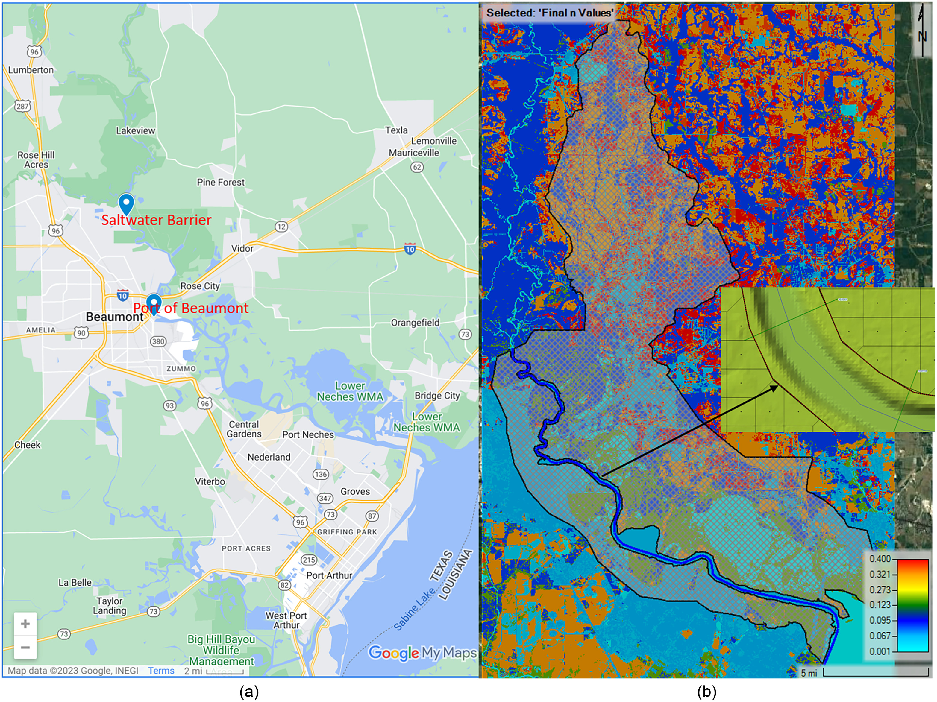
Fig. 1. Neches River tidal: (a) study area (map data ©2023 Google, INEGI); and (b) 1D and 2D model domain, grid, and Manning’s roughness coefficient of 2D area.

The river segment stretches for approximately 48 km (30 mi) from the Neches River Saltwater Barrier [Fig. 1(a)], which is 0.7 km (2,300 ft) downstream of the confluence of the Pine Island Bayou, to its outflow into Sabine Lake. Along the water edges, there are areas for filling spoil dredging materials. The waterway from the mouth of the river to the Port of Beaumont [Fig. 1(a)] is maintained by USACE, and it is currently dredged to 12.2 m (40 ft) deep and 122 m (400 ft) wide in order to accommodate marine traffic and large vessels (TPWD 1974).

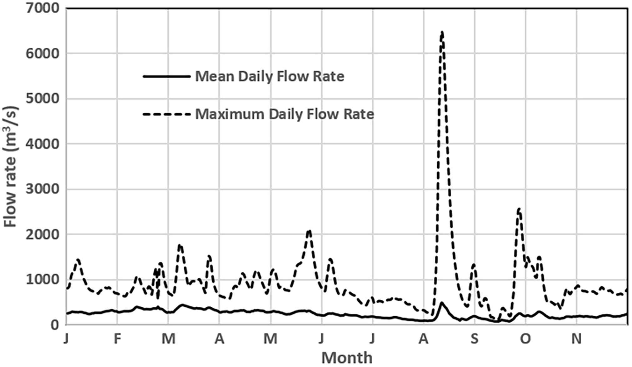
The Neches River Tidal section is subject to tidal influences that can reverse the flow direction of the river and cause significant cycles of approximately 24.84 h at USGS Gage Station 08041780 (Fig. 3) located at Neches River Saltwater Barrier. The available daily flow rates have been averaged to filter the tidal effect. The flow rate of

- 935 m^{3} / s

(

- 33,300 {ft}^{3} / s

; “–” means the reverse flow direction) on September 13, 2008, was caused by storm surge during Hurricane Ike. The maximum flow rate was

6,570 m^{3} / s

(

232,000 {ft}^{3} / s

) on September 1, 2017, with a gauge height of 6.60 m (21.56 ft) above the mean sea level (MSL) during Hurricane Harvey. The annual hydrograph for both maximum and mean daily discharge were developed with all available gauge data from 2004 to 2020 at Gage Station 08041780, as shown in Fig. 2.

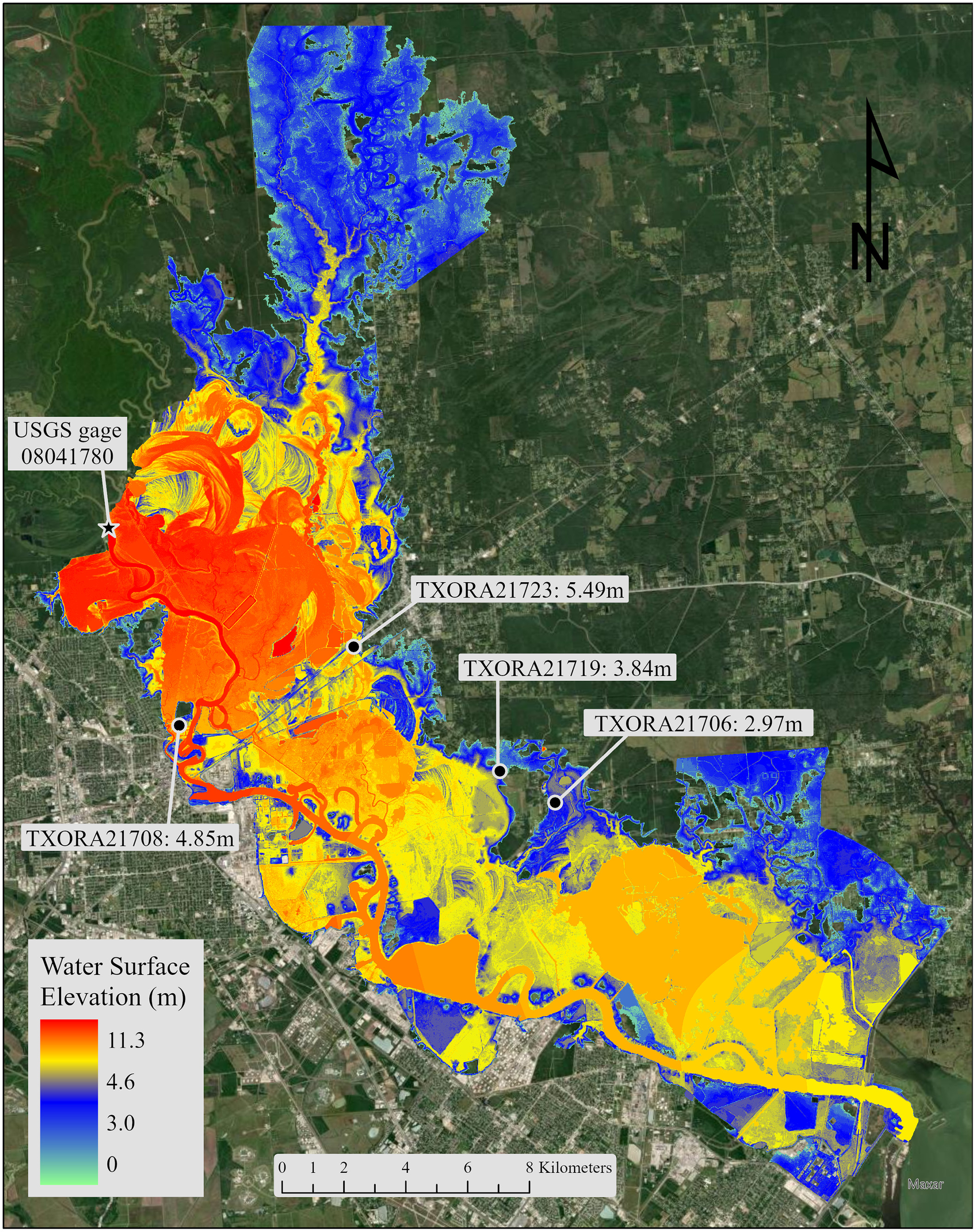
Fig. 2. The annual hydrograph between 2004 and 2020 for both maximum and mean daily flow at Gage Station 08041780.

Hurricane Harvey was recorded as the highest single devastating storm rainfall in the US, with more than 76.2 cm of rainfall in southeast Texas and a maximum total rainfall of 154.0 cm near the city of Nederland from August 25 to September 4, 2017 (NOAA 2017). The rainfall was estimated to correspond to a 1,000-year event and made it impossible for rivers and drainage systems to properly convey the water (Blake and Zelinsky 2018). Both USGS Gage Station 08041780 and the National Oceanic and Atmospheric Administration (NOAA) gauge located at the south of the Rainbow Bridge were damaged without official real-time data collected during Hurricane Harvey. Therefore, the flow rate at the USGS gauge and the water depth at the NOAA gauge were estimated after the event. Hurricane Harvey was identified as the only “no tidal affected” flood event in the Neches River Tidal section with both a model study (Maymandi et al. 2022) and field data (Lee 2022) due to the extreme flow rate from upstream. It flooded several watersheds and damaged one-third of the total structures (

\sim 110,000

structures) in Jefferson, Orange, Hardin, and Tyler counties (NOAA 2017). The geographic coordinates of four high-water mark sites in the Neches River Tidal watershed were obtained from the USGS Flood Event Viewer (USGS 2017) to generate a shapefile in ArcMap, as shown in Fig. 3. It illustrated four high-water marks above NAVD88 in Orange County, Texas (TXORA), and the inundation map in the watershed.

Fig. 3. High-water marks for Hurricane Harvey and inundation maps generated with ArcGIS. (Map data ©2023 Google.)

Material and Methods

Governing Equations for HEC-RAS Models

The 1D HEC-RAS river hydraulic model solving the conservation of mass and momentum is expressed in the following equations:

\frac{\partial A}{\partial t} + \frac{\partial (Φ Q)}{\partial x_{c}} + \frac{\partial ((1 - Φ) Q)}{\partial x_{f}} = 0

(1)

\frac{\partial Q}{\partial t} + \frac{\partial (Φ^{2} Q^{2} / A_{c})}{\partial x_{c}} + \frac{\partial [{(1 - Φ)}^{2} Q^{2} / A_{f}]}{\partial x_{f}} + g A_{c} [\frac{\partial H}{\partial x_{c}} + S_{f c}] + g A_{f} [\frac{\partial H}{\partial x_{f}} + S_{f f}] = 0

(2)

where

Q

= total flow;

A

= flow area;

Φ

= quotient of channel conveyance over the total conveyance;

H

= elevation of the water surface; and

S_{f}

= fraction slope, in which the subscripts

c

and

f

refer to the channel and floodplain, respectively.

The 2D HEC-RAS model solves the full Saint-Venant equations for the conservation of mass and is expressed in the following equations:

\frac{\partial H}{\partial t} + \frac{\partial (h u)}{\partial x} + \frac{\partial (h v)}{\partial y} + q = 0

(3)

\frac{\partial u}{\partial t} + u \frac{\partial u}{\partial x} + v \frac{\partial u}{\partial y} = - g \frac{\partial H}{\partial x} + v_{t} (\frac{\partial^{2} u}{\partial x^{2}} + \frac{\partial^{2} u}{\partial y^{2}}) - c_{f} u + f v

(4)

\frac{\partial v}{\partial t} + u \frac{\partial v}{\partial x} + v \frac{\partial v}{\partial y} = - g \frac{\partial H}{\partial y} + v_{t} (\frac{\partial^{2} v}{\partial x^{2}} + \frac{\partial^{2} v}{\partial y^{2}}) - c_{f} v + f u

(5)

where

h

= water depth;

u = x

-component of velocity;

v = y - component

of velocity;

q

= source/sink flux term;

v_{t}

= horizontal eddy viscosity coefficient;

c_{f}

= bottom friction coefficient; and

f

= Coriolis parameter. The model is solved to account for turbulence and the Coriolis effect and is capable of predicting dynamic flood waves, mixed flow regime conditions, and tidal environments. It can be used for spatially varied hydraulic analysis in cases with complex river geometries and flow patterns, especially when parameters such as flow direction and velocity are desired (Brunner 2016).

The coupled 1D/2D HEC-RAS model allows for direct feedback at each time step between 1D and 2D flow elements to enable the more accurate calculation of headwater, tailwater, flow, and any submergence that occurs at the hydraulic structure (Brunner 2016). The 1D reach was connected to the 2D flow area via a series of lateral structures aligned on the high ground of both banks of the river. These structures were modeled as broad-crested weirs to simulate overbank flows using the standard weir equation

d Q = C {(y_{w s} - y_{w})}^{2 / 3} d x

(6)

where

d Q

= structure flow over the length element

d x

;

y_{w s}

= water surface elevation;

y_{w}

= structure elevation; and

C

= weir coefficient. A hybrid discretization approach was considered to discretize the time derivatives with finite-difference approximation and discretize the spatial derivatives for grids with finite volume (Brunner 2016).

1D HEC-RAS Model Development

The FEMA BLE floodplain analysis (FEMA 2019) was implemented using the 10-m DEM, which is able to accurately represent bare earth surface elevations but generally lacks the ability to depict underwater surface profiles. Lacking bathymetric data may produce inaccurate flood inundation areas within the floodplain for certain flow rates, especially channels with dredged waterways. Therefore, the 1-meter DEM bathymetric data (USACE, personal communication) was merged with the 10-meter DEM using the mosaic tool in ArcMap by setting a priority for elevation values of raster data sets, including the underwater surface profile applying the LAST operator (ESRI 2019). The resampled DEM was exported from ArcMap and imported to RAS Mapper (Brunner 2016) using the NAD 1983 UTM Zone 15N projected coordinate system to develop the 1D HEC-RAS floodplain model. A total of 22 cross-sections, which began at the south end of the Saltwater barrier and concluded 1.6 kilometers upstream of the Rainbow Bridge, were revised to include the main channel and the 500-year floodplain as in the FEMA BLE model (FEMA 2019). Bank lines of the river were manually drawn roughly along the high ground of the river reach to compute the locations of bank stations. The National Land Cover Database (NLCD 2016) was used to determine the values of the left and right overbank Manning’s roughness coefficients by the Lotter Method (Brunner 2016) along each cross-section because NLCD 2011 and NLCD 2016 were almost identical for the watershed (NLCD 2011, 2016).

Coupled 1D/2D HEC-RAS Model Development

The coupled 1D/2D model was also implemented using the same resampled DEM as in the 1D model with the NAD 1983 UTM Zone 15N projected coordinate system. To establish the 2D flow area of the model, a shapefile containing the boundary of the Neches River Tidal watershed was imported into RAS Mapper to assist in accurately drawing perimeters for the floodplain and the main channel manually. The 2D flow areas encompassing a total of 96,847 computational

76.2 \times 76.2 - m

(

250 \times 250 - foot

) cells were generated, as shown in Fig. 1. No significant changes on water surface slopes and velocities were observed when applying a small cell size

30.5 \times 30.5 m

(

100 \times 100 feet

) because the watershed topographic consists of relatively low-lying land with gradual slopes. The 1D bathymetry data were defined by digitizing 57 cross-sections, which were drawn perpendicular to the flow direction along the reach using RAS Mapper. The geometry of each cross-section was determined using automated processes of RAS Mapper that create river centerlines, bank lines, and the underlying terrain file. Care was taken to ensure that each cross-section did not extend into the 2D flow area to avoid double counting the volume, as shown in Fig. 1(b). Land cover data for the watershed were obtained from the National Land Cover Database (NLCD 2016) data set and imported into RAS Mapper. Roughness coefficients for each land cover classification were manually defined following Liu et al. (2018). A spatially varied Manning’s roughness coefficient layer was then created in RAS Mapper, as shown in Fig. 1(b).

The total of 63 lateral structures of varying lengths were constructed along the banks to connect the 1D reach flow to the 2D flow area. Multiple lateral structures were used to accurately account for flow, improve model stability, and allow for weir parameter flexibility at different locations (Saksena et al. 2020). The geometry of each lateral structure was determined with RAS Mapper. A weir width of 0.61 m (2 ft) and weir coefficient of 0.5 were applied for most of the overbank lateral structures. Alternatively, a weir coefficient of 5.0 was applied at confluences, bends, and offshoots of the main river to more accurately simulate the increased flows experienced at these locations (Saksena et al. 2020).

Model Calibration and Validation

Channel Manning’s $n$ Calibration and Verification

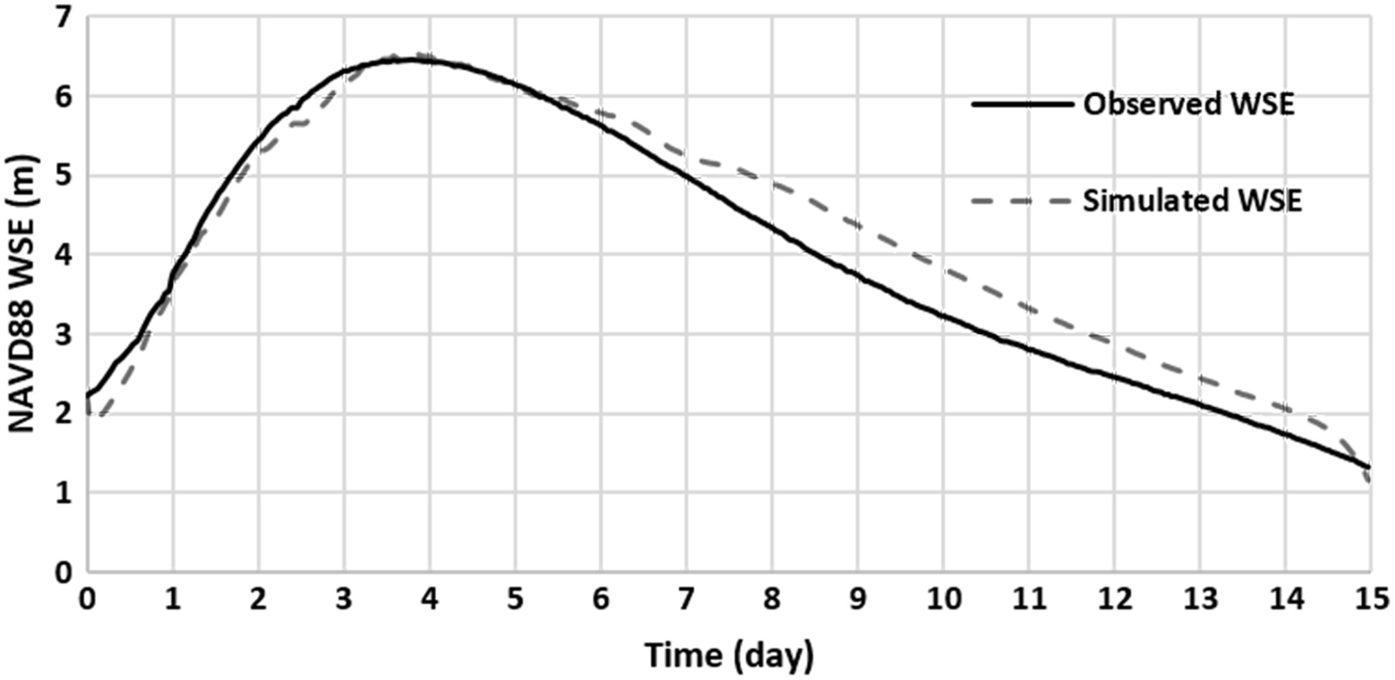
The channel Manning’s roughness coefficient was first calibrated under the steady flow conditions of the 1D model using streamflow and stage data collected at USGS Gage Station 08041780 as an upstream boundary condition. Steady flow profiles were generated for the five steady flow conditions in the range of

850 - 2,000 m^{3} / s

by applying the downstream normal flow with an average slope of 0.0001894 calculated from the bathymetry data. The average Manning’s roughness coefficient of 0.0524 was calculated and applied as a baseline roughness coefficient for unsteady flow conditions. Using the automated HEC-RAS flow roughness calibration tool, the downstream slope was adjusted manually between 0.0001890 and 0.0001900 until the calculated water surface elevations were close to the water surface elevations at Gage Station 08041780 for Hurricane Harvey from August 29 to September 12, 2017. As shown in Fig. 4, the coefficient of correlation of 0.9836 and coefficient of determination (

R^{2}

) of 0.9675 indicate good agreement between the simulated and recorded water surface elevation at Gage Station 08041780. The maximum simulated water surface elevation of 6.53 m occurred at 8 p.m. on September 1, 2017, whereas the maximum water surface elevation of 6.47 m was recorded at 7 p.m. on September 1, 2017. The roughness coefficients were then validated for 30 distinct flow rates using global optimization and the average error evaluation in the 1D HEC-RAS model and the 1D domain of the coupled 1D/2D model. The Manning’s roughness coefficient was determined in the range of 0.031–0.069, which was consistent with an excavated or dredged channel with a clean bottom and brush on the side (Chow 1959).

Fig. 4. Comparison between recorded and simulated water surface elevation at Gage Station 08041780 for Hurricane Harvey.

2D Flow Area Manning’s $n$ and Weir Coefficient Calibration

The 2D model was calibrated with high-water marks of Hurricane Harvey, as shown in Fig. 3. The after-event flow hydrograph from August 29 to September 6 was used as the upstream boundary condition with the initial 2.215 m to match the initial observed water surface elevation. Other initial observed water surface elevation values at field sites in Lee (2022) were also included. For the downstream, a normal depth boundary condition was applied with averaged friction slope because the river discharging to the Sabine Lake can be considered an open-ended reach, and the friction slope is typically hard to obtain ahead of time (Brunner 2016). Each 2D flow area had the dry initial condition, and the external boundary of the 2D domain was considered a Neumann boundary condition

\partial u / \partial n = 0

(Brunner 2016). In each cell, a value of 0.003 m (0.01 ft) was set for the cell volume filter tolerance, face profile filter tolerance, and face area-elevation tolerance, and a value of 2% (0.02) was set for the face conveyance tolerance ratio. An adjusted timestep based on the Courant number:

C = u Δ t / Δ x

was selected for time step control.

The 1D/2D model calibration process initially compared calculated maximum water surface elevations for Hurricane Harvey with that of the USGS high-water marks (Fig. 3) by increasing or decreasing 10%, 25%, 50%, 75%, and 100% of Manning’s roughness coefficients in the 2D area (Liu et al. 2018). Simulated maximum water surface elevations in the 2D domain were smaller than the recorded data under both increasing and decreasing roughness coefficients (Fig. 3) using a global calibration tool. Furthermore, the alteration of roughness coefficients also had a significant impact on the simulated stage height at Gage Station 08041780. Always resulting in smaller high-water marks under varied roughness coefficients implied that the model requires increasing weir coefficients of lateral structures to allow more flows to escape from the main channel into the 2D area. Weir coefficients were increased with 1% increments ranging from 1% to 20%. The errors between simulation and recorded data were calculated, and only cases with errors less than 15% are listed in Table 1. This indicates an increase of 10% of the weir coefficient was deemed sufficient for model calibration. The maximum error of 12.83% at the site of TXORA21723 (Fig. 3) demonstrated the calculated water depth was lower than the high marks. This is likely caused by the presence of the Interstate Highway 10 (IH 10) bridge because no bridge characteristic data was available to consider in the model development.

Table 1. Maximum water surface elevations (m) compared to high-water marks (m) with increased lateral structure weir coefficients of 1D/2D and 1D models

USGS high-water mark site	Recorded high-water marks (m)	Calculated maximum water depth (m)
		Weir coeff. increased in 1D/2D model					1D model
		0%	5%	6%	7%	10%	1D model
TXORA21708 (m)	4.85	3.77	4.53	4.56	4.56	4.62	4.63
% error		22.26	6.61	5.92	5.92	4.73	4.60
TXORA21723 (m)	5.49	4.19	4.71	4.74	4.77	4.79	4.60
% error		23.61	14.17	13.72	13.17	12.83	16.28
TXORA21719 (m)	3.84	2.89	3.92	3.97	4.01	4.08	2.67
% error		24.67	2.16	3.43	4.30	6.36	30.47
TXORA21706 (m)	2.97	2.10	2.87	2.88	2.91	2.92	1.92
% error		29.19	3.22	2.92	2.09	1.58	35.45

Model Scenario Development

First, the 1D HEC-RAS model applied compound flows by applying the upstream mean daily flows boundary condition (Fig. 2), and peak flow rates for the 10-year, 25-year, 50-year, 100-year, and 500-year storm events at each cross-section using regional regression equations developed by USGS (Asquith and Roussel 2009), as in the FEMA BLE model (FEMA 2019). The results from both models were analyzed to investigate the bathymetry effect on water depths and flood inundation areas.

Then, both 1D and 1D/2D HEC-RAS models were applied with flow rate data at USGS Gage Station 08041780 from Hurricane Harvey to calculate the maximum water depths and the flooding inundation maps. The model simulation results were compared with high-water marks and the inundation map area (Fig. 3) to illustrate the models’ accuracy.

Finally, the 1D/2D HEC-RAS model was applied with compound pluvial and fluvial flooding considering the 500-year flood event (Asquith and Roussel 2009) over the watershed along with the mean and maximum annual stream flow hydrograph at USGS Gage Station 08041780 (Fig. 2). Extreme flood events of increasing 10%, 25%, and 50% of the Hurricane Harvey flow rate at Gage Station 08041780 were considered not only to assess current design judgements of local agencies and stockholders but to provide inundation maps of the Neches River Tidal floodplain to consider when making decisions about mitigating flood impacts and improving resiliency.

Results and Discussion

Model Sensitivity on the Waterway Bathymetry

Water depths and flood inundation areas calculated using 1D HEC-RAS model were compared with those from the FEMA BLE model (FEMA 2019). The maximum water depths at the Port of Beaumont and flood inundation maps under different storm events and the percentage differences of both models are listed in Table 2. The results showed that bathymetric data integration reduced maximum water surface elevations in the waterway, and the difference decreased with the flood event year increasing. For example, the maximum water elevations (above the NAVD88) at the Port of Beaumont were 2.68 m with the FEMA BLE model considering a 10-year flood event and 1.27 m considering the mean daily flow rate and 10-year flood event with the greatest difference of 1.41 m; they were 4.20 m for a 500-year flood event in the FEMA BLE model and 3.70 m considering the mean daily flow rate and 500-year flood event with the least difference of 0.50 m. Therefore, the widened and deepened waterway provides extra storage to decrease the maximum water depth in the ship channel.

Table 2. Maximum water depth (m) at the Port of Beaumont and inundation areas (

{km}^{2}

) of floodplain for storm events using the FEMA BLE and 1D models

Flood event (year)	Maximum water depth at the Port of Beaumont (m)			Area ( ${km}^{2}$ )
Flood event (year)	FEMA BLE model	1D HEC-RAS model	% difference	FEMA BLE model	1D HEC-RAS model	% difference
10	2.68	1.27	52.61	162.55	129.16	$- 20.54$
25	3.05	1.79	41.31	168.90	155.85	$- 7.73$
50	3.31	2.22	32.93	173.14	172.55	$- 0.34$
100 minus	3.38	2.29	32.25	174.41	175.80	0.80
100	3.58	2.63	26.54	177.23	181.74	2.54
100 plus	3.80	2.90	23.68	180.21	185.83	3.12
500	4.20	3.70	11.90	186.10	195.96	5.30

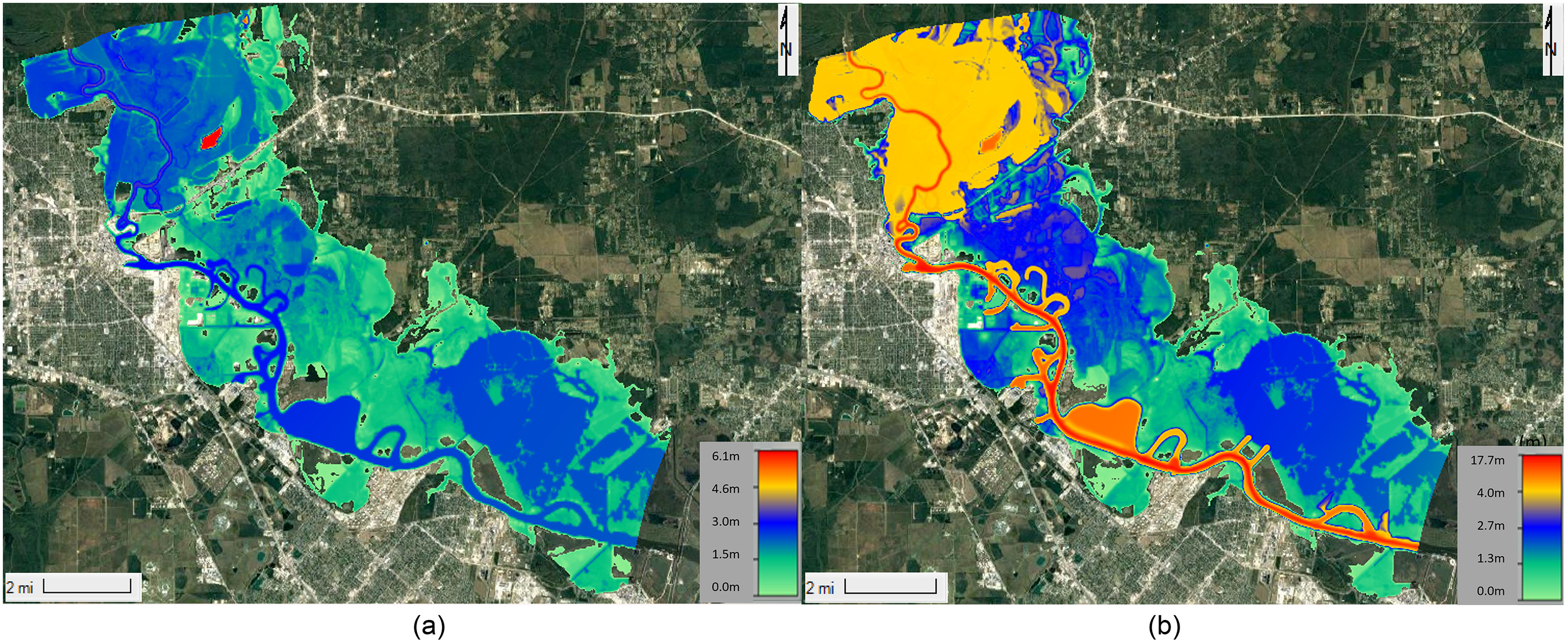
As shown in Table 2, the inundation map calculated by the 1D model was smaller than that calculated by the FEMA BLE model for 10-year, 25-year, and 50-year events but farther reaching than that for the 100 minus-year, 100-year, 100 plus-year, and 500-year events. The most significant reduction in inundated area can be seen in the case of the 10-year event, with inundated areas calculated for the event showing a 23% difference, or

33.40 {km}^{2}

(

13 {mi}^{2}

). The smallest difference between the two cases was determined in the 50-year event to be 0.34%, or

0.60 {km}^{2}

(

0.23 {mi}^{2}

). It is obvious that the waterway provides additional capacity to decrease the inundation maps for 10-year, 25-year, and 50-year flood events; however, the compound fluvial and pluvial flooding produces an impact that reverses the trend for the 100 minus-year, 100-year, 100 plus-year, and 500-year flood events. As shown in Fig. 5, the flood inundation area for the 500-year flood event using the FEMA BLE was smaller than the 1D model simulations at upstream areas above IH-10. Such results may be caused by complex hydrodynamics over the floodplain and main channel during large flooding events. As compared to the small Manning’s coefficient (0.001) in the FEMA BLE model for open water area in the main channel, the 1D HEC-RAS model was applied with higher Manning’s roughness coefficients (0.031–0.069), which could slow down the flow movement to increase floodplain flooding. In summary, flood inundation models are sensitive to bathymetric data and assumptions on Manning’s roughness coefficients. Therefore, such data are necessary for flooding management, and requisition of bathymetric data for other waterbodies in southeast Texas coastal region is recommended to local agencies and stakeholders.

Fig. 5. Five-hundred–year flood inundation map with (a) water depth calculated by the FEMA BLE model; and (b) 1D HEC-RAS model considering mean annual hydrograph. (Map data ©2023 Google.)

1D and Coupled 1D/2D Model for Hurricane Harvey

To assess model accuracy, both the 1D and coupled 1D/2D HEC-RAS models were compared by applying USGS Gage Station 08041780 data for the period between August 29 to September 6, 2017, during Hurricane Harvey because no tidal effect was identified during this time period (Maymandi et al. 2022; Lee 2022). The 1D and coupled 1D/2D models calculated the gauge depth at Gage Station 08041780 with

R^{2}

values of 0.7226 and 0.9076, respectively. The calculated high-water marks from the 1D model and the calibrated 1D/2D model are listed in Table 1. The error between recorded and calculated high-water marks from the calibrated 1D/2D model were in the range of 4.08%–12.83%, as shown in the column with the 10% weir coefficient increase in Table 1. The depth of 4.63 m with an error of 4.6% at TXORA21708 calculated with the 1D model was smaller than that calculated from the coupled 1D/2D model (4.62 m) with an error of 4.73%. However, significant errors were calculated as 16.28%, 30.47%, and 35.45% at TXORA21723, TXORA21719, and TXORA21706 with the 1D model, respectively. The results showed that the coupled 1D/2D model demonstrated overall higher agreement with both main channel gauge data and recorded high-water marks in the floodplain, as shown in Fig. 3.

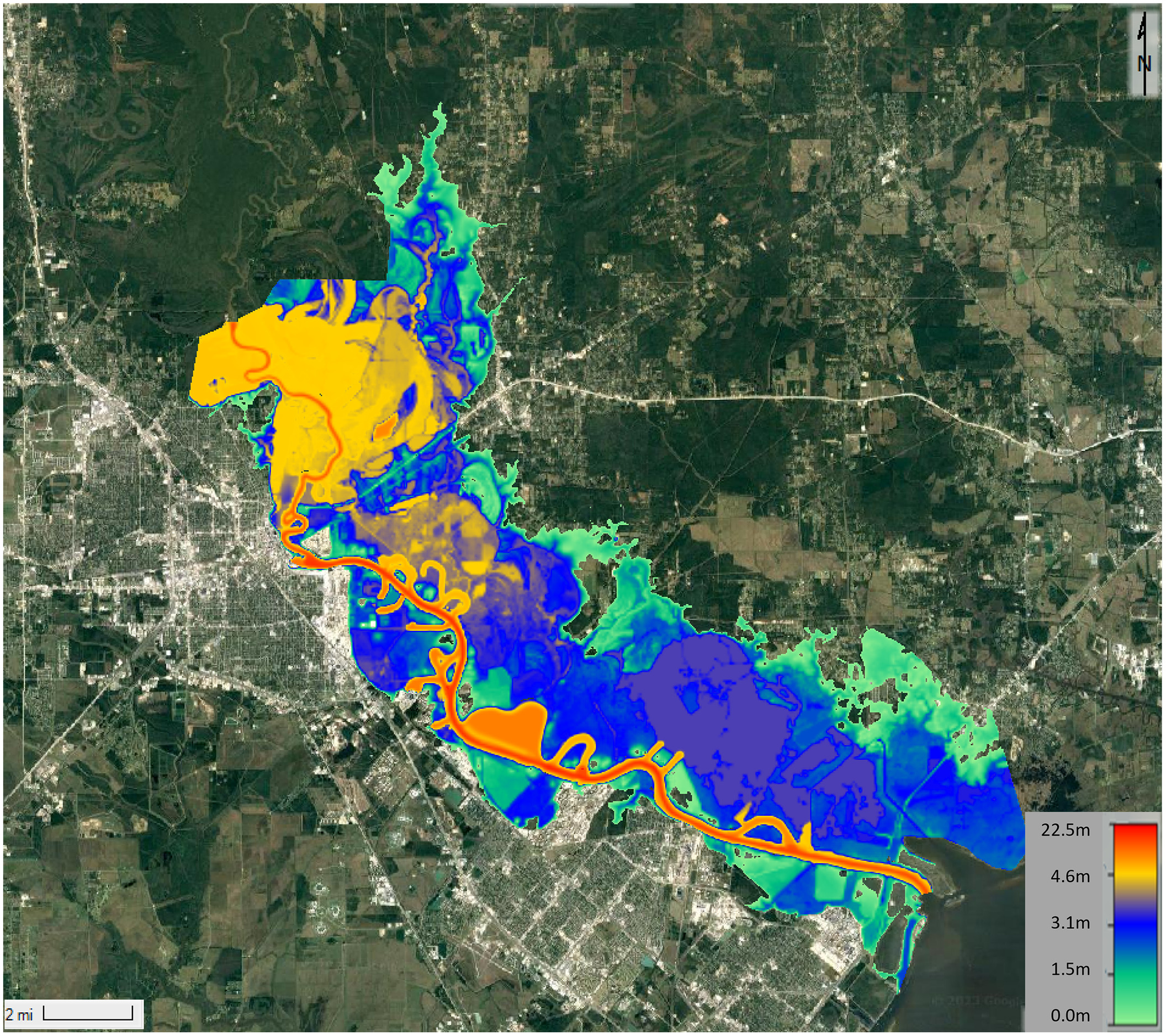
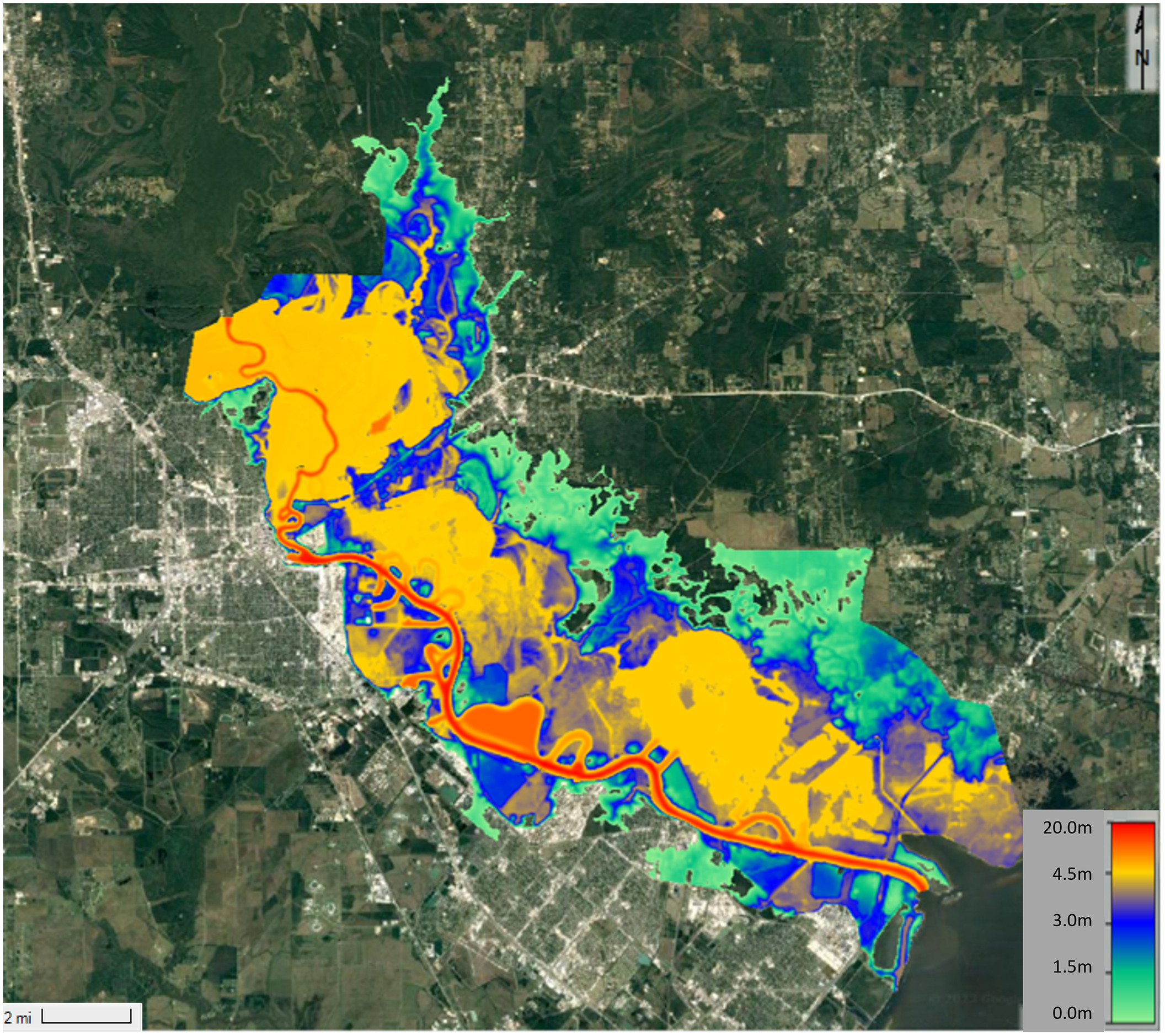
The 1D model resulted in an inundated area of 192.52 square kilometers (74.33 square miles), whereas the coupled 1D/2D model resulted in an inundated area of 268.98 square kilometers (103.85 square miles) for Hurricane Harvey, as shown in Fig. 6. Fig. 6(b) also shows the coupled 1D/2D model calculated more accurate inundation areas along the waterway where heavy industries are located and demonstrated the overflow to adjoined watersheds on both sides, for example, the cites of Beaumont, Port Arthur, Vidor, and Bridge City, as observed during the event (Lee 2022).

Fig. 6. Inundation map and water depth for Hurricane Harvey calculated by (a) the 1D model; and (b) the coupled 1D/2D model. (Map data ©2023 Google.)

Compared with the flood inundation maps in Fig. 3, both inundation maps in Fig. 6 showed less area at the north and west of the watershed. The inundated area of 327.38 square kilometers in Fig. 3 indicated a 70.00% and 21.70% increase from the 1D and coupled 1D/2D HEC-RAS model simulations, respectively. With the limited data available, both the 1D and the coupled 1D/2D model can only be developed to simulate the postevent case because event-based flooding simulation models with rain-on-grid assessment (Zeiger and Hubbart 2021) require time series rainfall and runoff data in the floodplain and gauge data in the main channel. Although the full 2D Saint-Venant Eulerian–Lagrangian method was applied in the 2D area for the coupled 1D/2D model, the postevent model may not have sufficient energy to transfer the river water to the overland area far from the channel. This could be caused by the high Manning’s coefficient of the natural forest land in the north and wetland in the west or smaller weir coefficients between the 1D and 2D domains. This difference can be attributed to the availability of high-water marks of the watershed for model calibration of 2D Manning’s and weir coefficients. Although the coupled 1D/2D model simulation underestimated the inundation area of the north and west area, it significantly improved the accuracy of the inundation map compared with the 1D model.

Coupled 1D/2D Model Results for Design and Extreme Flood Events

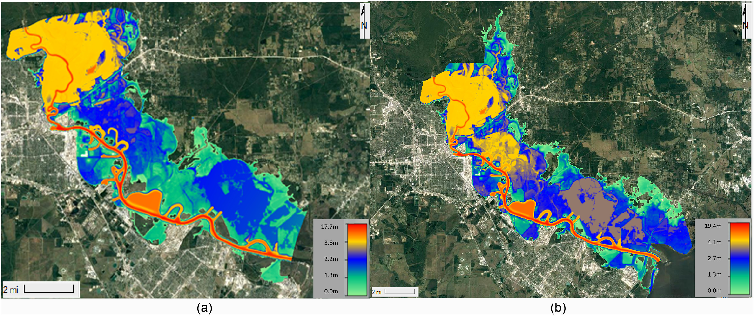
To generate inundation maps for design flood events, the calibrated 1D/2D model was used to simulate inundation maps for compound fluvial and pluvial flooding considering a 500-year flood event along with the mean or maximum annual stream flow hydrograph at USGS Gage Station 08041780 (Fig. 2), respectively. A maximum of 234.62 square kilometers was inundated by the 500-year flood event runoff under the mean annual hydrograph, whereas a maximum of 258.18 square kilometers (10.04% increase) was inundated when the maximum annual hydrograph was considered, as shown in Fig. 7. The maximum water surface elevations at the Port of Beaumont were calculated as 3.53 m for the mean annual hydrograph, 4.18 m for the maximum annual hydrograph, and 4.41 m for Hurricane Harvey. Compared with Hurricane Harvey, compound flooding estimations resulted in less area inundated and lower water depths at the Port of Beaumont. The results indicate that local hydrological and hydraulic design manuals may not be sufficient for extreme floods.

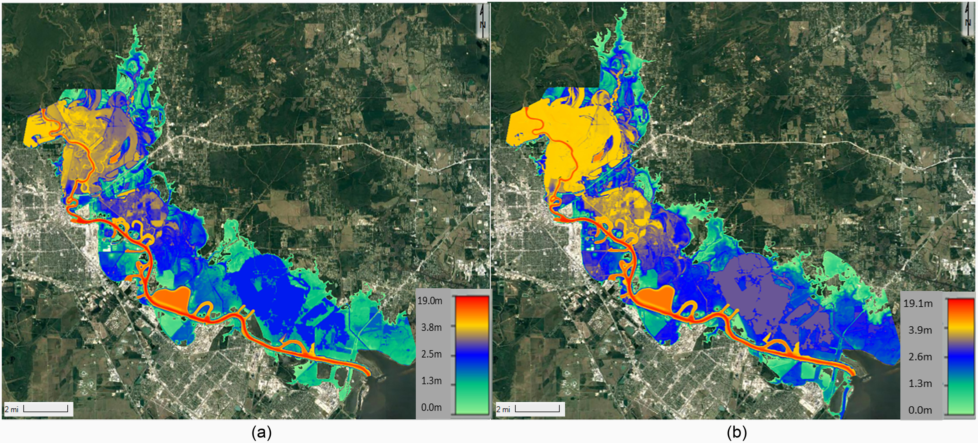
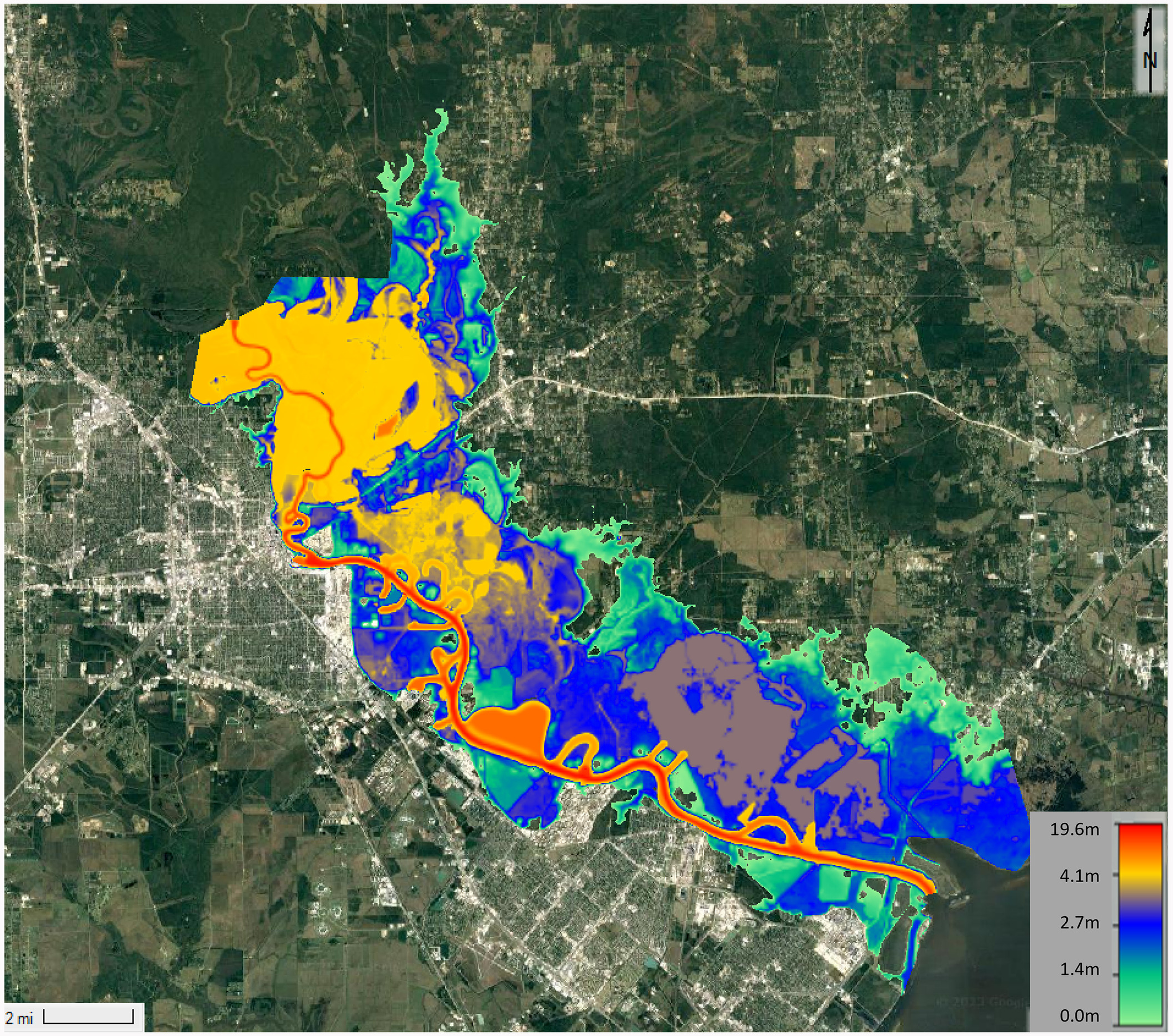
Fig. 7. Inundation map and water depth for the 500-year flood event calculated by the coupled 1D/2D model considering (a) mean; and (b) maximum annual hydrograph at Gage Station 08041780. (Map data ©2023 Google.)

Last, the coupled 1D/2D model was used to simulate extreme flood events when flows at the Saltwater Barrier increased by 10%, 25%, and 50% from that of Hurricane Harvey. The inundation area was calculated as 270.57 square kilometers for a 110% Harvey event, 272.48 square kilometers for a 125% Harvey event, and 317.28 square kilometers for a 150% Harvey event, as shown in Figs. 8–10. These areas increased by 0.6%, 1.3%, and 18% as compared with Hurricane Harvey, respectively. Compared with the inundation map of Hurricane Harvey, Fig. 8 showed more inundation area at the city of Pine Forest, south of the city of Vidor and along the waterway where many of the oil and gas industrial complexes are located. Fig. 9 showed even more inundation in the city of Beaumont, city of Port Arthur, and north of the city of Vidor compared to Fig. 8. Fig. 10 extends the flooded area far to the north of Pine Forest, crossing the watershed boundary into the city of Orangefield and reaching the watershed boundary in the cities of Nederland and Groves. The time-varied water depth of three extreme floods demonstrated that the increasing flood waters filled the floodplain faster and brought more overflow to pass over the watershed boundaries, increasing regional flooding. Inundation maps for extreme flood events implied that the drainage system in the city of Vidor, the city of Beaumont, Orange County, and Drainage District 7 of Jefferson County may require upgrading to mitigate future flood threats.

Fig. 8. Inundation map and water depth for the case of 110% Hurricane Harvey event. (Map data ©2023 Google.)

Fig. 9. Inundation map and water depth for the case of 125% Hurricane Harvey event. (Map data ©2023 Google.)

Fig. 10. Inundation map and water depth for the case of 150% Hurricane Harvey event. (Map data ©2023 Google.)

Maximum water depths of 4.49, 4.57, and 5.20 m were estimated at the Port of Beaumont for the 110%, 125%, and 150% Hurricane Harvey simulations, respectively. These are 0.08, 0.16, and 0.79 m higher than that during Hurricane Harvey, respectively. The calculated maximum water depths at four USGS high-water marks are summarized in Table 3. Although less than 0.30 m (1 foot) above high-water marks was calculated for both the 110% (0.01–0.11 m) and 125% (0.04–0.26 m) of Hurricane Harvey events, the 150% Hurricane Harvey event showed significant increases in the range of 0.79 to 1.43 m. Therefore, the current maximum design judgment of 0.30 m (1 foot) above high-water marks is only sufficient for the 110% and 125% Hurricane Harvey events but not recommend for events higher than 125% of the Hurricane Harvey event.

Table 3. Maximum water depth (m) at USGS high-water marks for extreme flood events

USGS high-water mark site	Calculated maximum water depth (m)				Increased depth compared with Harvey (m)
USGS high-water mark site	Harvey	110% of Harvey	125% of Harvey	150% of Harvey	110% of Harvey	125% of Harvey	150% of Harvey
TXORA21708 (m)	4.62	4.73	4.88	5.41	0.11	0.26	0.79
TXORA21723 (m)	4.79	4.91	5.04	5.57	0.12	0.25	0.78
TXORA21719 (m)	4.08	4.13	4.19	4.94	0.05	0.11	0.86
TXORA21706 (m)	2.92	2.93	2.96	4.35	0.01	0.04	1.43

Conclusion

The study developed 1D and coupled 1D/2D HEC-RAS models under different hydrological and hydraulic conditions to provide a more realistic perspective on possible flood threats and improve flood inundation mapping accuracy to mitigate flood hazards in the Neches River Tidal floodplain. Both models were calibrated or validated with the available flow rate data at USGS Gage Station 08041780 and recorded high-water marks during Hurricane Harvey.

Key points to take away from this study indicate that inundation maps are sensitive to the availability of bathymetric data, and different roughness coefficients in the floodplain and the main channel used in the 1D HEC-RAS model may not capture the complex nature of hydrodynamics. Therefore, obtaining bathymetric data integrated with DEMs for other waterbodies in the region is important for developing more realistic flooding inundation models. A coupled 1D/2D model provides a more realistic depiction of flood threats with the limited available data and is superior to the 1D model for producing accurate flood inundation maps of the Neches River Tidal floodplain, although the coupled 1D/2D model has limitations due to complex land cover and extreme flood conditions. The inundation maps for design and extreme flood events show that possible flood threats along the waterway and the cities of Beaumont, Port Arthur, Rose City, Vidor, and Bridge City and catastrophic region flooding cross multiple counties. Such valuable information can be useful for local agencies and stakeholders to assess flood vulnerability, make reasonable flood reduction investment decisions, and improve regional resiliency.

Overall, the coupled 1D/2D HEC-RAS model demonstrates plausible results and provides an effective model approach to better estimate flooding for similar regions with limited data availability. Although results from this exemplar flood inundation model application are telling, further model testing is recommended in the region as HEC-RAS developers continue to push the boundaries of HEC-RAS simulation capabilities.

Data Availability Statement

Some or all data, models, or code that support the findings of this study are available from the corresponding author upon reasonable request.

Acknowledgments

This material is based upon work supported by the NOAA-OAR-CPO-2019-2005530. Any opinions, findings, and conclusions or recommendations expressed in this material are those of the author(s) and do not necessarily reflect the views of the NOAA. We also appreciate partial student support from the Center for Resiliency at Lamar University.

References

Asquith, W. H., and M. C. Roussel. 2009. Regression equations for estimation of annual peak-streamflow frequency for undeveloped watersheds in Texas using an L-moment-based, PRESS-minimized, residual-adjusted approach: Scientific investigations report 2009–5087. Reston, VA: USGS.

Abstract

Introduction

Study Area and Data

Material and Methods

Governing Equations for HEC-RAS Models

1D HEC-RAS Model Development

Coupled 1D/2D HEC-RAS Model Development

Model Calibration and Validation

Channel Manning’s n Calibration and Verification

2D Flow Area Manning’s n and Weir Coefficient Calibration

Model Scenario Development

Results and Discussion

Model Sensitivity on the Waterway Bathymetry

1D and Coupled 1D/2D Model for Hurricane Harvey

Coupled 1D/2D Model Results for Design and Extreme Flood Events

Conclusion

Data Availability Statement

Acknowledgments

References

Information

Published In

Copyright

History

ASCE Technical Topics:

Authors

Affiliations

Metrics

Citations

Download citation

Figures

Other

Share

Copy the content Link

Share with email

Share

Request Username

Create a new account

Change Password

Password Changed Successfully

Verify Phone

Congrats!

Channel Manning’s $n$ Calibration and Verification

2D Flow Area Manning’s $n$ and Weir Coefficient Calibration