Laboratory Measurements of Hydraulic Jacking Uplift Pressure at Offset Joints and Cracks
Publication: Journal of Hydraulic Engineering
Volume 150, Issue 4
Abstract
Hydraulic jacking is a serious threat to concrete spillway chutes, demonstrated by the catastrophic spillway chute failure at California’s Oroville Dam in 2017. To improve the understanding of uplift pressure and joint flow developed at open, offset joints and enable design and evaluation of anchors, drain systems, and joint remediations that could help prevent such failures, laboratory tests were performed in a supercritical flume furnished with a model joint where the gap width to offset height ratio was varied over a range. The tests included measurement of boundary layer velocity profiles approaching the joint. Uplift pressures were normalized to the velocity head near the boundary, which is related to the depth-wise velocity profile exponents determined in the experiments and can be estimated for field applications from the chute friction factor. The normalized uplift varies with the joint aspect ratio and the flow depth to offset height ratio. The new relations reduce the uncertainty of modeled uplift pressures by a factor of 2.87 over previous methods. Example applications demonstrate practical upper limits for potential uplift pressure. Subsequent articles will address discharge into offset joints, the dissipation of uplift via drainage, and the effect of different methods for remediating existing offsets to reduce uplift.
Practical Applications
Concrete spillway chutes develop cracks and must necessarily be constructed with joints, both of which are prone to displacement over time that may create offsets into the flow. Flow striking such offsets is brought suddenly to rest, similar to a pedestrian tripping on a sidewalk crack. The local stoppage of flow at the offset creates dangerously high pressures that can be injected into the foundation, leading to erosion beneath the slab and potential uplift failure, often called ‘hydraulic jacking’. This mechanism has caused several notable failures including the Oroville Dam spillway in 2017. Protection against such failures is usually provided by a combination of the weight (thickness) of the slab itself, anchors that hold the slab down, and subsurface drains that reduce the buildup of pressure. This paper provides experimentally based equations for predicting uplift pressure to enable effective design of new spillways and evaluation of existing spillways. The new equations are significantly more accurate than previous methods because they account for the roughness of the chute surface and the reduced flow velocity near the boundary. Subsequent papers will address flow rate through joints, pressure dissipation by drainage, and methods for treating existing offsets to reduce potential uplift.
Introduction
Hydraulic jacking can occur when high-velocity flow in a spillway chute or similar structure passes over an open joint or crack that is offset into the flow. Offsets can develop through differential movement of the foundation (e.g., expansive or contractive soils, consolidation or frost heave), or due to a damaged concrete surface (a spall) located adjacent to a joint. Open joints may exist in older spillways that were not constructed with waterstops, or in newer spillways due to misinstallation or failure of waterstops.
Flow hitting an offset is brought suddenly to rest (stagnation), converting kinetic energy into high pressures at the floor of the channel that can propagate through the joint or crack and force water under the slab. Suction on the top surface of the downstream slab also occurs due to flow separation just downstream from the offset but is neglected in this article because the magnitude of this pressure change is slight compared to the potential increase below the slab and is ultimately limited by the vapor pressure of water. It should be noted that cavitation induced by offsets can also cause severe spillway damage, but hydraulic jacking can occur at flow velocities well below those needed to cause cavitation. High pressures entering a joint can extend under the slab for significant distances, especially if there are voids in the foundation below the slab. If pressures are sufficiently high, total forces capable of lifting (jacking) the slab further up into the flow are possible, which amplifies the problem and can lead to explosive failure. The jacking or peeling off of rock slabs by high-velocity turbulent flow is also a process that occurs in unlined spillway chutes and plunge pools (Bollaert 2012; George 2015; Pells 2016). Additionally, flow that gets through the joint or crack and continues under the slab may cause erosion of the foundation if not contained by a drainage system. This can create or enlarge voids, progressively extending the area exposed to uplift pressure, which increases the chance for uplift failure and creates the possibility of slab collapse into the void after flow has ceased.
It should be noted that the terms ‘hydraulic jacking’ and ‘hydrojacking’ are also used in the geotechnical engineering community in connection with pressurized tunnels drilled through a pervious rock mass (e.g., USACE 1997). If insufficient overburden is present, internal stresses originating from the pressurized tunnel may be sufficient to jack open existing fractures in the rock. If stresses exceed the tensile strength of the rock mass, new fractures may be created, which is described as ‘hydraulic fracturing’ (Amberg and Vietti 2015).
Case Histories and Defensive Measures
Either failure mode described above destroys the integrity of the chute lining, which can allow rapid erosion of underlying material. Headcut erosion following the initial failure of the chute lining at Oroville caused concern for possible uncontrolled release of the reservoir; use of the previously untested emergency spillway to minimize further damage to the main spillway also caused headcutting that prompted an evacuation order affecting about 180,000 people. Repairs and upgrades to the spillways eventually cost about $1.1 billion. Another recent failure attributed to hydraulic jacking was the fifth drop structure on the St. Mary Canal in Montana in May 2020, which was taken out of service for the entire 2020 irrigation season while two of the five drop structures on the project were rebuilt (Irrigation Leader 2020, 2021). Other recent uplift failures include spillways at Eping Dam in China (China Observer 2021), Bukan Dam in Iran (Bahramifar et al. 2022), Toddbrook Reservoir Dam in the United Kingdom (Hughes 2020; Mauney undated), and Rhymney Bridge 2 reservoir in Wales (Hughes and Williamson 2014). Other documented historic failures include Big Sandy Dam spillway (Wyoming) in 1983 and Dickinson Dam spillway (North Dakota) in 1954 (Hepler and Johnson 1988; Trojanowski 2004; Frizell 2007). A near-failure of the spillway at Hyrum Dam (Utah) (Trojanowski 2008) occurred when flow through open joints created large voids below the slab, and a similar near-failure incident at Fairbairn Dam in Australia took place in 2011 (Foster et al. 2016), although the Fairbairn case may have been related more closely to stilling basin pressure fluctuations than uplift at offsets within the chute. Masonry-lined spillways are also prone to uplift failures as demonstrated by cases in the U.K. at Ulley Dam in 2007 (Hinks et al. 2008), Boltby Dam in 2005 (Charles et al. 2011), and Butterly Dam in 2002 (Chesterton et al. 2018). Given these recent failures, rehabilitation projects and designs that can prevent uplift failure are being actively discussed in recent literature (Gilbert et al. 2023; Lux et al. 2023; Smith et al. 2023; Vensel et al. 2023).
The typical thickness of concrete spillway slabs has increased over time, ranging from about 0.2 to 0.3 m (0.75 to 1.0 ft) before the 1960s to about 0.3 to 0.61 m (1 to 2 ft) more recently (personal communications with practicing spillway engineers: Patrick Maier, Bureau of Reclamation; John Trojanowski, Trojanowski Dam Engineering Ltd.). The weight of the slab provides a first defense against uplift failure, but even a submerged 0.61-m (2-ft) thick slab on a flat slope can be displaced by a net uplift pressure head of only 0.86 m (2.8 ft) and a slab on an incline is even more easily displaced; such uplift pressures can easily be generated by flow stagnation at an offset. Thicker slabs provide space for installing two layers of reinforcement and allow adequate embedment of anchor bars. Other defensive measures include proactive design of joints with offsets slightly away from the flow so that small differential movements can be tolerated without immediately creating dangerous offsets, keyed or doweled joints to prevent differential movement, waterstops to prevent water intrusion, anchor bars to secure slabs to the foundation, and drainage systems to alleviate pressure buildup and safely convey flow out of the foundation. Design of the latter two features requires accurate estimates of uplift pressure and flow rates through affected joints. In spillways with existing offsets, mitigation may also include beveling and grinding down offsets or modifying joints to restore sealants or waterstops.
The Oroville failure was carefully investigated by an Independent Forensic Team (IFT 2018). The 1960s-era design lacked waterstops and keyed or doweled joints, had insufficient anchorage due to age-related corrosion and weak foundation materials (anchors embedded in soil-like materials rather than competent rock), and probably had insufficient drainage. Many older spillways have similar characteristics. The IFT evaluations of anchorage and drainage systems carried significant uncertainty due to limited experimental studies of offset joint hydraulics in either laboratory or field conditions. The IFT report presented calculations of estimated stagnation pressure at offsets of various heights. Those estimates were informed by previous experimental studies and used estimated boundary layer velocities at the tip or mid-height of offsets determined with a basic open-channel flow velocity profile equation (Rouse 1945). This approach had not been experimentally verified and did not include any influence of the gap width. The IFT report also provided estimates of seepage flow through open joints of various widths based on a simple orifice equation, considering the driving head to be only the hydrostatic pressure associated with the depth of flow in the chute and assuming a fully vented condition below the slab. This approach neglected the effect of offset height and the increased driving head created by stagnation of flow at an offset.
Previous Research
Only two previous experimental studies of hydraulic jacking are known, both performed at the Bureau of Reclamation (Reclamation) hydraulics laboratory in Denver, Colorado (Johnson 1976; Frizell 2007). The problem has been of great interest to Reclamation because of its many older spillways and chutes constructed on soil or rock foundations. These structures are more prone to hydraulic jacking than chutes integrated into mass concrete arch or gravity dams, since the concrete spillway lining is a relatively thin veneer over a weaker and variable foundation. Hydraulic jacking failure modes are commonly considered in Reclamation’s risk assessment studies.
The study by Johnson (1976) was aimed at supercritical chutes associated with small canal systems. It used a 2.44-m (8-ft) long, 0.15-m (0.5-ft) wide open-channel laboratory flume limited to velocities of (). Documentation is limited, but the flume was probably level. Measurements of static uplift pressure and dynamic pressure fluctuations were made at a model joint with variable offset height and gap width, sealed to prevent any net flow through the joint.
Frizell (2007) used a level water tunnel supplied by a high-head pump to generate velocities up to () approaching an adjustable joint, with tests of square, chamfered, and radius joint edges. Measurements of static uplift pressure were made, but there were no measurements of dynamic pressures. Measurements of flow rate through joints were also attempted, but most of the flows were determined indirectly with unknown backpressure conditions below the joints and are thus unreliable with little predictive value. Both studies showed that uplift pressure was directly dependent on chute velocity, and that uplift increased with the offset height and decreased with increasing gap width. The Johnson study reported uplift pressures relative to the mean velocity head in the channel but presented these dimensionless values as functions of absolute (dimensional) velocities and joint dimensions. The Frizell study reported dimensional uplift pressures as functions of joint dimensions and flow velocities. Unfortunately, these presentations of the data do not facilitate application to other scales, joint configurations, or flow conditions. Neither study measured or estimated the boundary layer flow properties in the experimental facilities, although both discussed the potential influence of the boundary layer and suggested that such measurements be included in future studies. Frizell (2007) did some limited velocity vector mapping within and above the joint for one joint configuration ( offset with gap) using particle image velocimetry (PIV) and commented on the potential influence of the observed boundary layer.
Investigation of past failures has been limited until the Oroville failure, with the best early documentation provided by Hepler and Johnson (1988) for the Dickinson and Big Sandy failures. The Oroville and Dickinson failures occurred well upstream from the toe of each chute, away from any possible tailwater influences. The Big Sandy failure was closer to its stilling basin, but probably still above the zone of influence of the basin’s hydraulic jump. Wahl et al. (2019) reviewed literature on stilling basin failures in zones affected by the turbulent flow of the hydraulic jump, but this problem is driven by much different flow mechanics than mid-chute failures. Smith (1995) describes an alternate uplift failure mode at the toe of a chute where supercritical flow enters a stilling basin. In this failure mode, hydrostatic pressures created by the tailwater depth in the basin cause uplift behind the chute lining and below the toe of the chute that cannot be counterbalanced by the depth of the incoming supercritical flow. The driving forces in this case do not develop from an offset into the flow, but only from seepage through joints, cracks, or drainage systems within the basin lining. Eductors that utilize offsets away from the flow to draw water out from beneath the lining through a venturi effect can help to protect against this mode of failure (Smith 1995).
In the first phase of the present study, Wahl et al. (2019) combined and reanalyzed data from the Johnson (1976) and Frizell (2007) laboratory studies. Adjustments of the Frizell (2007) data were made to account for effects of the water tunnel experimental setup, which increased the measured pressures due to factors that would not be present in an open-channel environment. This analysis showed that the normalized uplift pressure head illustrated in Fig. 1 was related to the dimensionless joint aspect ratio, , aswhere = gap or slot width; = height of the offset into the flow; = increased pressure head compared to the hydrostatic pressure associated with the flow depth; = mean velocity in the chute; and = acceleration due to gravity. The normalized uplift pressure head was shown to vary, with significant scatter, from about 0.1 to 0.7 within the range down to , increasing with decreasing . It was difficult to discern whether smaller values of might lead to still larger uplift pressures, but Eq. (1) represents that trend, indicating an upper bound of for . The reanalysis also attempted to develop relations between uplift pressure and boundary layer velocity similar to those used in the Oroville forensic analysis, although neither previous study directly measured boundary layer velocities. As a result, boundary layer velocities could only be estimated for the previous studies, and the resulting relations exhibited more data scatter than Eq. (1).
(1)
Sánchez (2022) used the ANSYS Fluent computational fluid dynamics (CFD) model to simulate the experimental work of Frizell (2007) and two open-channel flow situations with 30° and 45° slopes. For sealed conditions with no flow through joints, the results matched the Frizell experimental work closely, with maximum deviations of 6%. For vented conditions the deviations were up to 15%, which may be due to the unknown backpressure conditions and joint flow rates in the Frizell study. The open-channel simulations at the two slopes yielded almost identical uplift pressures, indicating that slope is an insignificant factor in the relation between flow velocity and the stagnation pressure occurring within a joint of fixed geometry.
Following the reanalysis of the Johnson (1976) and Frizell (2007) data sets, Reclamation constructed an experimental facility designed to address questions posed by IFT (2018) and Wahl et al. (2019). The objectives of the experimental work are as follows:
•
Develop relations to boundary layer velocity that can improve estimates of uplift pressure,
•
determine practical upper limits for uplift pressure associated with small values of ; and
•
develop experimentally supported relations for predicting flow rates through joints and cracks.
The first two objectives are addressed in this article. Test data related to flow rates through joints and cracks will be presented in a subsequent article.
Experimental Facility
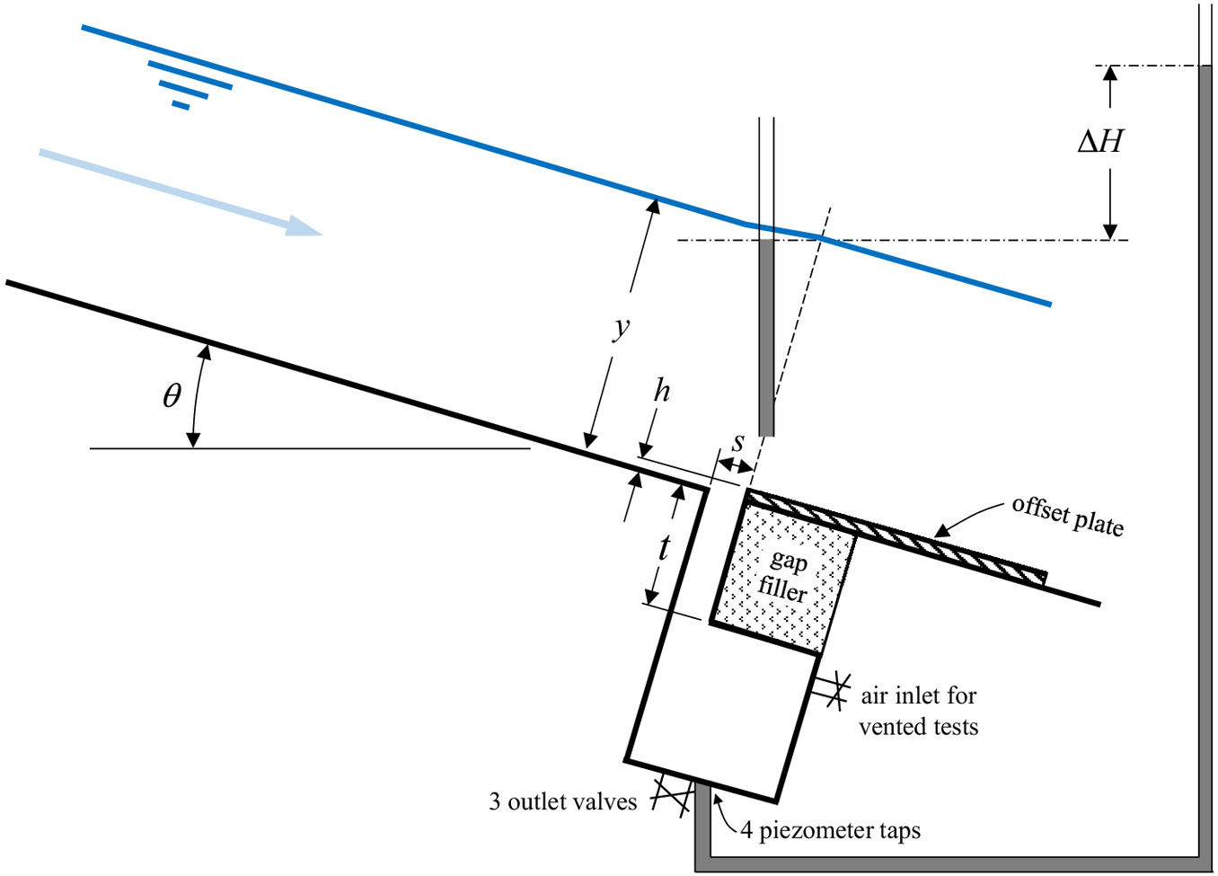
The new laboratory facility was placed into service in early 2021 at Reclamation’s hydraulics laboratory in Denver, Colorado. The 0.61-m-wide (2-ft) smooth acrylic flume on a fixed 15° slope is equipped with an adjustable spillway joint located near the downstream end (Fig. 2). The approach distance to the joint is 8.76 m (28.75 ft), producing a well-developed, uniform (normal depth) or gradually varied flow profile, depending on discharge. Flow enters through a jet box (Schwalt and Hager 1992; Frizell and Svoboda 2012) that can give the incoming flow a high Froude number if desired. The flume is supplied from the laboratory’s fixed pumps and venturi meter flow measurement systems, which include meters from 3- to 14-in. diameter calibrated against a weight-based tank. Uncertainty of discharge measurements from this system is generally or better.

The model spillway joint consists of a 57-cm by 7.62-cm (22.5-in. by 3-in.) chamber in the flume floor that spans most of the channel width. The chamber extends 44 cm (17.25 in.) below the flume floor and is equipped with three 50-mm (2-in.) diameter outlet valves at the bottom and a 19-mm (.) diameter air inlet valve near the top of the chamber. Plates installed downstream from the joint create offsets into the flow to simulate a displaced spillway slab, and a portion of the chamber can be filled with solid materials to vary the width of the gap and the slab thickness, . Tested offsets were constructed from a variety of materials, including brass, aluminum, high density foam, expanded PVC panels, and marine plywood. Care was taken to ensure that materials were water resistant and suitably rigid to avoid deformation during tests in which large uplift forces were generated. Gap widths and offset heights were measured for each configuration using digital calipers or feeler gauges and a machinist’s height gauge.
For vented testing, joint discharge from the chamber was measured with a 90° V-notch weir that operates in a partially contracted flow condition for most flow rates. The weir box is equipped with a stilling well and Lory Type-A hook gage with vernier scale measurement precision of 0.0003 m (0.001 ft). Flow calibration of the weir is based on the Kindsvater–Carter weir equations as described in the Water Measurement Manual (Bureau of Reclamation 2001).
Tests have been performed at chute discharges from 0.01 to (0.35 to ), producing unit discharges up to () and mean flow velocities at the tested joint up to about (). Froude numbers at the joint location have ranged from about 6.7 to 13, where is the flow depth just upstream from the offset as shown in Fig. 1. Reynolds numbers have ranged from to , where is the hydraulic radius and is the kinematic viscosity. This puts all tests at the edge of or within the zone of fully turbulent flow.
Joints have been tested with offsets ranging from 0.75 mm () up to 12.6 mm () and gap widths ranging from about 0.45 mm (0.018 in.) up to 76.2 mm (3 in.). Tests have spanned ratios of 0.044 to 32—a ratio of , or almost three orders of magnitude. Tests have included square-edged joints, chamfers, radius edges, skewed and tilted joint orientations, and other configurations. Most tests have considered situations where the downstream side of the joint is offset perpendicularly into the flow, as shown in Fig. 1. One test was conducted with a very wide gap and a small offset away from the flow, and only slight uplift pressure was measured in the joint. Most tests have used the smooth acrylic approach flow surface of the constructed flume, but a few tests have been performed with a range of artificially roughened floor overlays that change the boundary layer velocity profile. The slab thickness, , (i.e., length of the flow path through the joint) was varied from about 5 to 28 cm (2 to 11 in.), but uplift pressure was independent of for sealed-joint conditions. The effect of joint thickness on flow rate through a joint is addressed in a subsequent article.
Velocity profiles have been measured using a 1.32-mm-diameter (0.052-in.) stainless steel Pitot tube installed with its inlet port 70 mm (2.75 in.) upstream from the chamber. This position was fixed for most of the study, so the distance from the tube’s inlet port to the face of the offset changed as the gap width was varied. This location was found in trials to be far enough upstream that measured velocities were unaffected by the offset but close enough to minimize changes in flow conditions between the Pitot tube and the offset. Although this particular Pitot tube also includes a static pressure leg just above the dynamic tube, it did not give consistent indications of flow depth; better results were obtained by integrating the velocity profiles and calculating the flow depth by continuity. Velocity profiles included at least 5 up to 10 points between the channel bed and water surface, and the position of the Pitot tube within the water column was determined from the Lory Type-C point gage used to position the tube with a vernier scale precision of 0.1 mm (0.00033 ft). Flow depths were also validated against approximate flow depths determined from an acoustic water level sensor mounted above the water surface. The Pitot tube calibration was checked using a facility in the laboratory in which the integrated velocity profile measurements across a flow nozzle were compared to discharge measurements from the laboratory venturi meters. Pitot tube measurements were made at the centerline of the channel for all tests, and lateral surveys of velocity were made early in the study to develop correction factors to convert centerline velocities to width-averaged mean velocities. These factors were adjusted as needed for joint configurations that did not span the full width of the 57-cm-wide (22.5-in.) chamber. Differences between centerline and width-averaged velocities were about 3.5% for joints spanning most of the channel width.
Pressures within the spillway joint were sensed via four manifolded piezometer taps equally spaced along the centerline of the bottom of the chamber, with the outlet valves centered between the taps (Fig. 1). All Pitot tube measurements and uplift pressure measurements from the model spillway joint were obtained visually from a nearby manometer board equipped with 3-mm () glass tubes and 4.8-mm () clear vinyl tubing. All measurements from the differing tube sizes were adjusted for capillary rise.
Test Procedure and Measurements
For each test condition, the velocity profile above the spillway chute surface (Fig. 3) was measured from the floor to near the water surface using the Pitot tube, and the mean uplift pressures within the modeled joint were measured at the manometer board. The maximum uplift pressure was measured with the chamber below the joint sealed (outlet valves closed) so that there is no net flow through the joint. Next, the valves on the bottom of the chamber were incrementally opened to permit flow through the joint, and the reduced uplift pressure and associated flow rate through the joint were measured (Fig. 2). Estimated uncertainties for the measured data are shown in Table 1.

| Parameter | Estimated uncertainty | Measurement method |
|---|---|---|
| Chute discharge, | Laboratory venturi meters | |
| Chute velocity, | Pitot tube | |
| Chute velocity near bed (below ) | Pitot tube | |
| Chute velocity above | Pitot tube | |
| Flow depth | Continuity equation using , | |
| Uplift pressure | () | Manometer board |
| Joint discharge | Sharp-crested V-notch weir | |
| Gap width | () | Calipers or feeler gage |
| Offset height | () | Machinist’s height gage |
Velocity Profiles
All velocity measurements were fit well by power curve equations in which or , where is dimensionless velocity normalized by the mean velocity and is dimensionless distance from the boundary normalized by the flow depth. The quality of the power curve fits indicates that the flow was well developed at the joint test station. The fitted profiles were used to determine the average velocity and flow depth. The exponent of the power curves varied with flow depth, corresponding to changes in the relative roughness and effective friction factor of the chute. The value of decreased with decreasing flow depth and decreased significantly for the handful of tests run with roughened floor conditions, consistent with expectations. It should be noted that the closest Pitot tube measurements to the boundary are located far above the likely upper bound of the viscous sublayer and buffer zone, and all offset heights tested were also many times taller than the thickness of the viscous sublayer. Thus, it is reasonable to represent the entire velocity profile with a single power law equation. Although the form of the velocity profile indicates well-developed flow, it should also be noted that the flow at the tested joint location was still accelerating for most tests; plots of lengthwise profiles of velocity, depth, and Froude number indicated that uniform, normal-depth flow was only reached at the joint for unit discharges less than about 0.107 m3/s/m (1.15 ft3/s/ft). This is consistent with potential applications for this research since many spillways operating at high discharges experience accelerating flow for much of their length.
Experimental measurements of uplift pressure have been normalized in this research with respect to the boundary layer velocity head, which depends on the velocity profile exponent in . In the laboratory studies, has been determined by fitting to the Pitot tube velocity measurements. For prototype application, has previously been related to the Darcy friction factor, . Nunner (1956) used data from Nikuradse (1933) and Laufer (1954) along with his own experiments to develop the empirical relation , which can also be expressed as . Subsequent investigations by many others, well summarized by Karim and Kennedy (1987), produced more complex expressions that have often been reduced to a relatively simple relation found in several newer references (e.g., Chen 1991; Chanson 1994):where is the von Kármán constant. Such a relation will allow to be determined for prototype chutes without the need for direct velocity profile measurements.
(2)
Detached versus Attached Flow
A prominent feature of an offset into the flow is that flow will fully detach from the chute floor if the offset is large compared to the flow depth (Fig. 4). If the jet breaks up in the air before landing again in the chute, it will remain detached, since air can penetrate the disintegrated jet. For deep flows, full jet breakup does not occur, and the jet remains attached to the floor since the flow entrains any air that is present and additional air cannot get under the jet. This is the usual condition for most prototype spillway flows, but both conditions can be produced in the lab over a large range of flows. The attached jet condition can be established by starting at a large discharge that produces naturally attached flow, and then reducing the discharge. Alternately, at low flow rates, the detached jet can be physically forced down to the floor using a handheld deflector plate, and, once attached, the flow will remain attached down to a relatively small flow rate. If detached jet conditions are again desired, the flow can be easily detached by momentarily disrupting the flow near the offset face with an obstruction. Attached jet conditions were the primary focus and baseline condition for the study, but measurements were made for both conditions whenever possible; for a given flow condition approaching a joint, jet detachment leads to greater uplift (up to about 8% of the approaching velocity head). For each joint configuration, tests were performed from high discharges down to the lowest discharge that would allow for attached flow. A few tests were run at discharges so low that only detached flow could occur.

Test Conditions Summary
Testing has been conducted for a wide variety of joint configurations and flow conditions. This paper presents results from the following:
•
Regular joints: square-edged joints oriented perpendicular to the flow direction and normal to the chute surface, with smooth acrylic chute floor (39 different ratios, 240 test runs with attached flow, 197 test runs with detached flow).
•
Rough-floor: tests of regular joints conducted with a roughened chute floor surface upstream from the joint (four ratios, six tests with attached flow).
Analysis and Results
Table S1 in Supplemental Materials provides the uplift pressure data for all tests. The attached-flow data were used initially to test Eq. (1) (Wahl et al. 2019) and other simple relations between and the normalized uplift pressure head . Similar trends between the variables were present, but uplift pressures measured in the new study consistently averaged about 3% lower than those predicted by Eq. (1). This matches an expectation that uplift pressures in the Johnson and Frizell studies may have been biased high for two reasons. First, the short approach distances to the test sections [1.5 m (5 ft) and 2.4 m (8 ft), respectively] probably produced incomplete flow development with higher boundary layer velocities than a fully developed flow. Second, jet detachment likely occurred in at least some of the tests. The Johnson (1976) study in an open channel flume with velocities up to () and offset heights as large as 38 mm (1.5 in.) seems likely to have produced some detached jet conditions, depending on flow depths, but the report makes no mention of it. Unfortunately, flow depths for each test were not reported, although they were probably 0.2 m (0.67 ft) or less based on the reported gate size entering the flume. Jet detachment is unlikely to have occurred in the Frizell (2007) water tunnel study due to the confinement of the water surface and the lack of a route for air to reach the detachment point.
The trends of the new data are well represented by a simple equation with an alternative form from that of Eq. (1):
(3)
This is consistent with the trend still evident in the new and broader data set for the uplift pressure head ratio to not exceed about 0.6, even for values as low as 0.045. However, there is still significant data scatter around this relation, with variation up to (Fig. 5) and a root-mean-square (RMS) error value of 3.59% of for the attached-flow tests of regular joints. In addition to this scatter, simple uplift versus relations do not provide a means for incorporating boundary layer effects, which makes them poorly suited for applying smooth-boundary laboratory test results to prototype chutes with significant surface roughness.

New Uplift Pressure Head Relations
Several potential empirical equations were investigated to relate normalized uplift pressure head to other experimental parameters singly and in combination, including , the velocity exponent , the Froude number, several Reynolds numbers using different velocity and length references, and several variations of roughness Froude numbers (Wahl 2023) utilizing the offset height, . Parameters used to normalize the uplift pressure head included the mean channel velocity head and the velocity head at various discrete positions within the boundary layer, such as the mid-height and tip of the offset. Relations were also investigated based on the concept of determining the distance from the bed to the hypothetical streamline in the velocity profile whose velocity head matched the measured uplift pressure head. However, none of these empirical methods were satisfactory over the full range of tests.
Ultimately, the most useful relations for modeling and predicting uplift pressure were based on the normalized uplift pressure head , where is the velocity head of the flow in the boundary layer integrated between the chute floor and the tip of the offset. This can be determined from the velocity profiles measured with the Pitot tube.
Relating back to the mean channel velocity is convenient and provides insight into the relation between the velocity head of the boundary layer and that of the bulk flow. We follow the same development process given by Chow (1959) for the familiar energy coefficient or Coriolis coefficient, , which is used to calculate velocity head using the mean velocity, . The energy coefficient is given by , where is the velocity through a differential area and is the total flow area. Integrating from the bed to the water surface, this relates the total kinetic energy of the water passing through the area to that calculated for a uniform velocity through the same area. If the velocity profile is described by a power curve as shown in Fig. 3 with , integration yields . Changing the limits of integration to cover only the zone from the channel bed to the offset height, , the result isand the velocity head of the flow between the chute floor and the tip of the offset is . The coefficient is the ratio of the velocity head in the boundary layer, , to the simple velocity head calculated from the average chute velocity, . Values of in the uplift research flume varied from about 5 for shallow flow in roughened channels up to 10 for deeper flow with the smooth acrylic floor. Thus, the range of was about 1.025 to 1.08. Values of range from zero to , depending on the relative offset height, (assuming never exceeds ). For the jet striking an offset to remain attached to the chute floor in these tests, the relative offset height had to be less than about 0.33 to 0.5, or alternately the relative submergence of the offset, , had to exceed 2 to 3. The smallest attached-flow value of was about 2 with ; for cases of large , was as small as 0.16.
(4)
Fig. 6 shows the normalized uplift pressure head as a function of for selected values; approximately 40 different combinations of and were tested, but for clarity this figure shows data for only a few cases. For a given value of the normalized uplift pressure increases nonlinearly with , and for any given the normalized uplift pressure increases nonlinearly with decreasing , as shown in Fig. 7. The curves fitted to the data in Fig. 6 all use the equation form:which can be transformed into
(5)
(6)


Eq. (6) is linear and convenient for regression analysis to determine the fitting parameters and . [A form was also considered in which the numeral 1 in the denominator of Eq. (5) was replaced with a third fitted parameter, , but this offered too many degrees of freedom and did not produce useful results.] This equation indicates that for each value of the normalized uplift asymptotically approaches a value of 1.0 for large values of . The asymptotic limit is visually apparent for the smaller values in Fig. 6 but less obvious for large . However, the quality of the curve fits demonstrates that Eq. (5) provides a good representation of the behavior for all within the range of conditions that could be tested. Fig. 8 shows data from all tests of regular joints with the smooth acrylic floor.

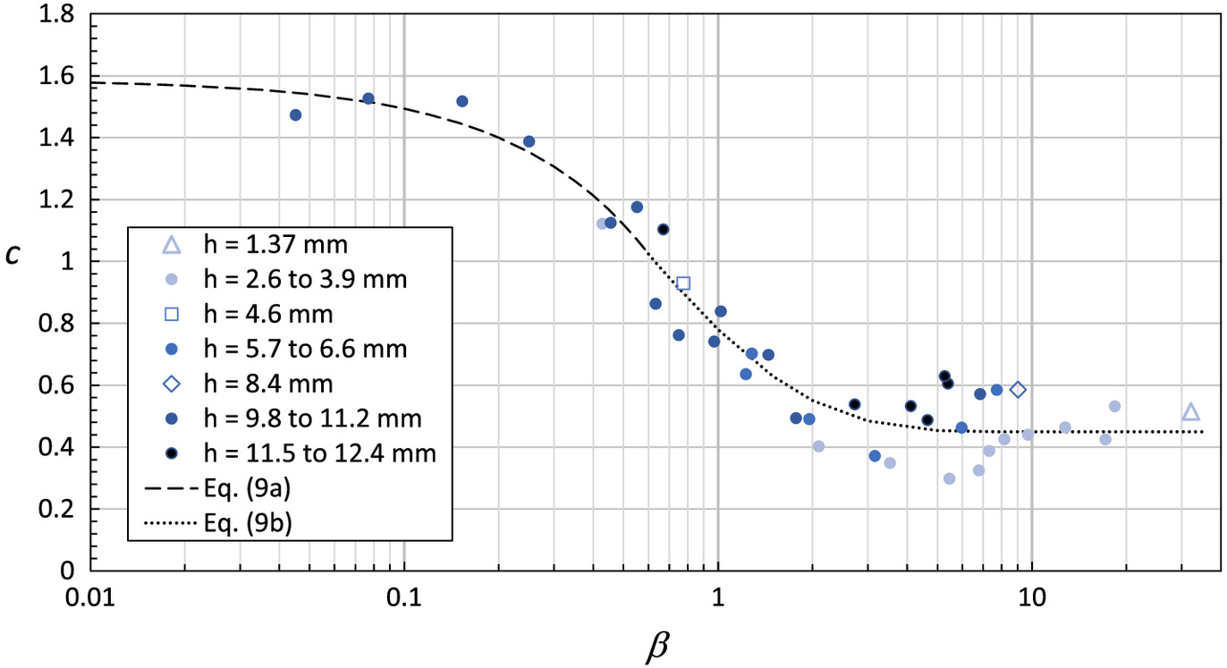
The curve fitting parameters and in Eq. (5) both vary as functions of , as shown in Figs. 9 and 10. Values of can be represented with a single curve:while values of are represented by two curveswhere = base of natural logarithms. Increased scatter of and is noticeable in Figs. 9 and 10 for approximately . The source is evident in Fig. 8 where there is significant crossing of the fitted curves in the region of to 8 and to 0.35. These crossing curves with differing values of and correspond to tests of joints with similar ratios, but different offset heights. The curves on the left side of this region are for large offsets (up to about ), which could only be tested at low ratios for even the largest possible discharges, while the curves on the right side of the region are obtained from offsets as small as 3 mm that could only be tested at larger ratios due to small flow depths and detachment at very low discharges. This behavior can be considered a scale effect caused by the interaction of the chute flow with the circulation that develops within the joint, below the plane of the chute surface. The shear between these flows creates a shear boundary layer that reduces the velocity of at least some of the flow impacting the offset. The thickness of this layer increases with the distance that the chute flow travels across the gap. When is small (offset height large relative to the gap width), this layer is thin in comparison to the offset height, so the effect is minimal. For larger the effect is increased as the layer becomes thick in comparison to the offset height. The effect begins gradually, becomes quite noticeable by about , and continues to be visible up to about . The maximum gap width in the test facility and limits on accurate construction and measurement of extremely small offset heights make it impractical to test a significant range of offset heights for larger values of , but if such testing could be performed the effect should continue to be seen for all larger values of .
(7)
(8a)
(8b)

To better understand the development of this shear layer, velocity profiles were measured above open gaps at incremental distances, , downstream from the start of the gap, with no offset installed. Profiles were measured above a 76.2-mm (3-in.) wide gap for two discharges, designated Q3 () and Q13 (), and a 38.1-mm (1.5-in.) wide gap at a third discharge, designated Q9 (). Normalizing velocity with respect to the mean velocity in the chute, , and distances across the gap and above the chute floor with respect to the gap width, and , the velocity profiles exhibit a consistent behavior shown in Fig. 11, with measurements over the narrower gap omitted from the figure for clarity. Velocity over the gap is gradually reduced from the initial chute velocity profile in a layer whose thickness grows linearly and is equal to about 11% of . Over the first third of the gap, the entire layer is a transitional zone in which the top of the layer matches the initial chute velocity, and the bottom has a growing velocity reduction compared to the original profile. Over the last two thirds of the gap, the shear layer continues to grow, composed of the transitional layer and a thickening lower layer in which the velocity is reduced uniformly by about 12% from the original chute velocity. Tests with the narrower gap showed similar trends, and the velocity reduction in the lower layer remained about 12%, appearing to be independent of the gap width. The lower part of the shear layer exhibits a similar slope on the log–log plot to that of the original profile, while the transitional zone has a steeper gradient of velocity versus depth. As the scale of the offset and gap change, the shear layer has a nonlinear effect on uplift pressure due to the variation of the velocity reduction factors. Offsets of any scale with the same value have the same proportion of their height influenced by the shear layer, but for small-scale offsets the transitional portion makes up all or most of the layer while larger-scale offsets become dominated by the lower portion with its greater velocity reduction.

Eqs. (5), (7), and (8) provide a generalized method for predicting the normalized uplift pressure for a joint with a given value of . To test the method, Eqs. (7) and (8) were used to determine values of and as functions of rather than obtaining and by curve-fitting to individual test data. Eq. (5) was then used to compute the normalized uplift, . To enable a more direct comparison to the previous evaluation of Eq. (3), which computed , we define the velocity head of the full flow as (since can be determined when the velocity profile is known) and convert values of to equivalent values of using
(9)
This also provides a more realistic evaluation of relative errors than a comparison of values, since large errors in are less significant when the offset height and are small.
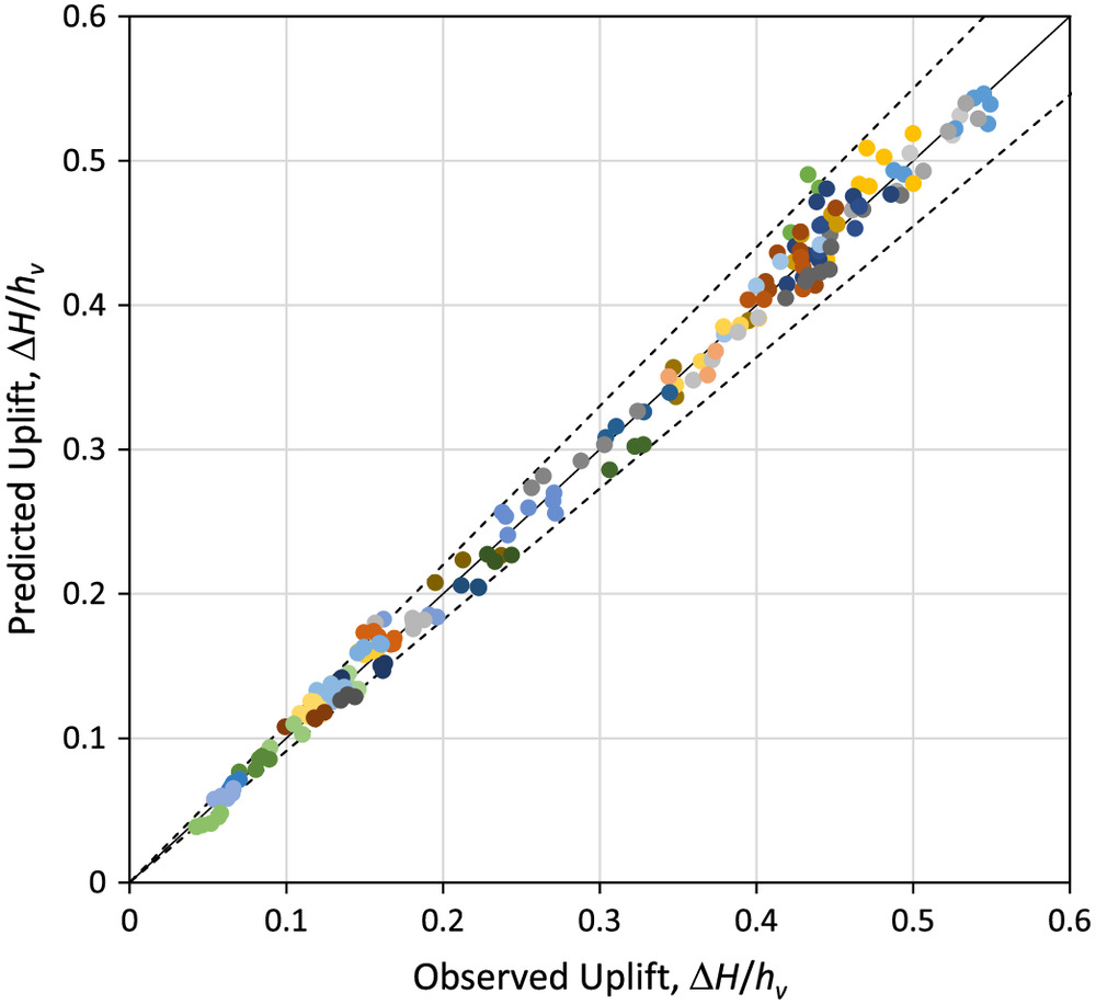
Fig. 12 shows predicted versus observed values of for the full set of regular joint tests. The majority of predictions are inside of the error band, with most of the larger errors occurring in the zone influenced by the scale effect discussed previously. The root-mean-square (RMS) average of errors for the complete data set is 1.25% of , reduced by a factor of 2.87 from the RMS errors of Eq. (3) applied to the same data.
Effects of Chute Roughness
Tests conducted with the smooth acrylic floor exhibited significant effects of changing roughness and variation of the boundary layer velocity profile, since relative roughness varied with discharge and flow depth over a range of about . This caused to vary from about 6.8 to 9.9. To test an even wider range of conditions, surface roughness was added to the chute upstream from the joint using several different treatments: 80-grit sandpaper (approx. sand particle diameter) adhered to the acrylic floor for a distance of about 1.2 m (4 ft) upstream from the joint; fabricated roughness panels with discrete triangular ridges perpendicular to the flow direction; and a 3.6 m (12 ft) length of expanded metal screen. Velocity profiles measured near the beginning, intermediate, and downstream points of the roughened sections showed that new well-developed velocity profiles existed at the joint, accurately represented by power curve equations with reduced values of between 5.0 and 5.8 and reduced velocity magnitudes near the floor consistent with the increased roughness. Although these profiles exhibited a power curve shape over the full depth that could be measured, it should be emphasized that uniform flow (i.e., normal depth) was not achieved for these tests; the flow was still decelerating at the tested joint, in contrast to the accelerating flow that existed for high-flow tests with the smooth acrylic floor.
Table 2 shows results of the rough-floor tests and compares observed uplift to that calculated by three methods: Eqs. (5)–(9) using the value fitting the measured velocity profile; Eqs. (5)–(9) using that represents a relatively smooth chute; and Eq. (3), which relates uplift only to without considering boundary layer velocity conditions. The generally lower errors for the first method compared to the second and third show that accounting for the effects of roughness on the velocity profile significantly improves the agreement between predictions and experimental results. Note that errors are expressed as percentages of to give an indication of their magnitude in relation to actual pressure differences. If errors were computed relative to observed values of or the percentage differences would be considerably larger in most cases. These results validate the use of the new uplift pressure equations for a wide range of channel roughness conditions, even though the relations were developed primarily from smooth-channel tests, and they demonstrate that through reduction of , additional roughness clearly causes a significant reduction of uplift pressure.
| (mm) | (mm) | () | (cm) | (m/s) | (m) | Observed | Eqs. (5)–(9) with measured N | Eqs. (5)–(9) assuming | Eq. (3) | |||||
|---|---|---|---|---|---|---|---|---|---|---|---|---|---|---|
| Predicted | Error (% of ) | Predicted | Error (% of ) | Predicted | Error (% of ) | |||||||||
| (m) | (m) | (m) | (m) | |||||||||||
| 2.4 | 10.9 | 4.61 | 0.390 | 5.99 | 6.51 | 5.09 | 2.33 | 0.183 | 0.185 | 0.11% | 0.398 | 0.436 | ||
| 2.4 | 10.9 | 4.61 | 0.237 | 4.17 | 5.68 | 4.98 | 1.78 | 0.165 | 0.156 | 0.319 | 0.332 | |||
| 3.0 | 6.4 | 2.14 | 0.598 | 8.08 | 7.40 | 5.78 | 2.97 | 0.407 | 0.410 | 0.11% | 0.709 | 0.835 | ||
| 4.7 | 37.8 | 8.00 | 0.137 | 3.53 | 3.90 | 5.61 | 0.82 | 0.071 | 0.071 | 0.01% | 0.102 | 0.108 | ||
| 20.7 | 7.2 | 0.35 | 0.393 | 6.26 | 6.29 | 5.00 | 2.18 | 0.918 | 0.849 | 1.116 | 0.926 | |||
| 20.7 | 7.2 | 0.35 | 0.746 | 9.34 | 7.99 | 5.01 | 3.52 | 1.325 | 1.197 | 1.733 | 1.497 | |||
Note: Estimates are made accounting for boundary layer via measured velocity profile exponent, , using assumed value of typical of smooth chutes, and using Eq. (3) (Wahl et al. 2019), which does not consider boundary layer conditions.
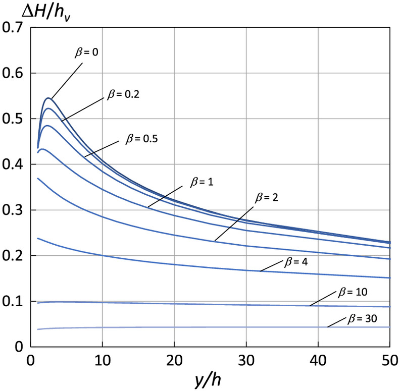
Maximum Normalized Uplift Pressures
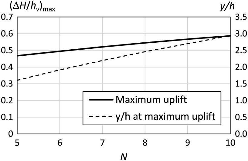
Eqs. (5)–(9) can also be applied to a range of hypothetical conditions to investigate the maximum possible uplift pressure head. The experimental data suggest an upper limit of about 60% of . To apply the equations, a value of must be assumed. Arbitrarily taking as a representative value (approximate median of observed values in the lab tests), Fig. 13 is obtained. Figs. 6 and 8 showed that uplift pressure normalized to approaches an asymptotic limit of 1.0 for large , but at these conditions is also quite small and the offset is exposed to boundary layer velocities that are much less than the mean velocity, so less uplift should be expected. Fig. 13 confirms this and shows that when normalized to the mean velocity head, peak uplift pressure head is about , occurring near ; uplift also drops significantly for larger values of y/h that are typical of design discharge conditions. Over the range of to 10 the peak varies almost linearly from to and the location of the peak varies almost linearly from to 2.94 (Fig. 14).
Additional Uplift for Detached Jets
Eqs. (5)–(9) predict the uplift pressure head for jets that remain attached to the chute floor downstream from an offset into the flow. If the flow detaches from the floor due to a large offset that forces the flow into the air so that the jet breaks up before landing downstream, the uplift pressure will be increased due to the momentum thrust needed to deflect the jet. Some of the increased pressure on the chute floor is transmitted into the joint. Increases measured experimentally were as large as 20% of , 8% of , or 60% of the attached uplift. While the increases are significant for a given flow condition, detached uplift pressure will rarely be a design concern for most spillways, since even greater uplift will occur at large flow depths and velocities that produce attached flow. Procedures for determining whether flow will detach from the floor and empirical relationships for estimating the additional uplift are provided in Supplemental Materials.
Determining for Field Application
The results presented thus far enable the calculation of uplift pressures when the ratio of an offset joint or crack is known along with the flow depth, mean velocity, and exponent of the flow profile, . Eq. (2) was introduced as a potential means for determining as a function of the Darcy–Weisbach friction factor, , and the experimental data provide the opportunity to refine this relation.
For each of the tests performed with the smooth acrylic floor, friction factors, , were computed at the joint using the Colebrook–White equation (i.e., the Moody diagram) as presented by Morris and Wiggert (1972), and these were used to compute the friction slope . Fig. 15(a) shows that for unit discharges less than or equal to (), the friction slope matches the chute slope, which indicates that uniform flow has been reached. The values were calculated assuming surface roughness , which is slightly lower than suggested reference values for glass, drawn tubing, and other smooth materials, but fits very well. Values of and were completely insensitive to smaller values of , indicating that the flow is at the limiting hydraulically smooth condition. For larger flow rates, the flow is still accelerating, so the friction slope is flatter than the chute slope and increasing in the downstream direction. The points in Fig. 15(a) that are scattered vertically, parallel to the axis, correspond to tests for which the jet box was used to provide higher velocity flow at the entrance to the chute. For these tests the flow came closer to reaching uniform conditions and in a couple of instances appears to have reached it, but only the low-flow points are confidently indicated here as uniform flow. For the largest flow rates, the jet box was pressurized and increasing the flow velocities entering the chute even when fully open.

Fig. 15(b) shows the relation between and the exponent determined from the velocity profiles. Both uniform and gradually varied flow cases follow the curvewhich is an adjustment of Eq. (2), with still taken to be 0.4. The quantity is close to the empirical value of originally determined by Nunner (1956). Previous discussions of Eq. (2) and other variants in the literature suggest that the connection between and may only be consistent for uniform, nonaerated flow (e.g., Chanson 1994), but the relation appears here to be good for both uniform and gradually varied flows within the range of these tests. Even when uniform flow does not exist, the friction factor seems to reliably indicate the magnitude of turbulent energy transfer from the boundary and its effect on the velocity gradient and the flow profile shape. This is reinforced by the fact that , where is the shear velocity , a parameter with velocity units that relates bed shear stress to fluid density and indicates the intensity of turbulent flow activity in the boundary layer. A few slightly aerated flows occurred during this test program, especially when the jet box was being used to strongly accelerate the inflow; this may explain the few data points at low values of the friction coefficient (high flows) that fall below the curve in Fig. 15(b).
(10)
With Eq. (10) available, the process for applying the laboratory results to real spillways involves the following steps:
•
Use an appropriate spillway water surface profile calculation tool such as SpillwayPro (Wahl and Falvey 2022) to obtain the depth, mean velocity, and friction factor at stations of interest.
•
Use the friction factor and Eq. (10) to estimate , the exponent of the velocity profile.
Application Example
The Oroville spillway forensic report (IFT 2018) estimated theoretical stagnation pressures for a range of potential offset heights at the time of initial failure when flow was being increased from 850 to (30,000 to ) in the 54.46-m-wide chute (178.67-ft). The calculations were based on theoretical estimates of the boundary layer velocity profile but did not consider the influence of the gap width; they could be considered to represent only the stagnation pressure at the face of the offset, not the fraction that would actually propagate into a joint.
Table 3 compares the IFT values to estimates of uplift pressure in and below the joint computed with Eqs. (5)–(8), and (10) for a range of gap widths and the same offset heights considered by the IFT. The calculated uplift pressures are about 15% to 35% of the IFT’s stagnation pressure estimates, with the greatest differences at larger gap widths. Although lower, these pressures are still large enough to have caused slab movement considering the poor anchorage and drainage conditions found in the forensic investigation. For example, the 6.31 m uplift head for the 25 mm offset and 6.4 mm gap is sufficient to displace an unanchored 4.6-m (15-ft) thick concrete slab. The upper bound of possible uplift pressures is indicated by the column for zero gap width. Obviously, a gap width that is truly zero would not allow for the transmission of pressure into the joint, but a gap slightly larger than zero can lead to the development of full uplift pressure if there is no drainage below the joint. Example calculations for the case of highlighted in bold in Table 3 are given in the Appendix.
| Offset height, [mm (in.)] | Uplift pressure head, [m, (ft)], for different gap widths, | Forensic estimate of stagnation pressure head (IFT 2018) [m (ft)] | ||||
|---|---|---|---|---|---|---|
| () | () | () | (1 in.) | |||
| 3.2 () | 1.96 (6.44) | 1.93 (6.34) | 1.83 (5.99) | 1.59 (5.23) | 1.25 (4.11) | 8.66 (28.4) |
| 6.4 () | 2.91 (9.53) | 2.89 (9.49) | 2.83 (9.29) | 2.62 (8.60) | 2.20 (7.23) | 11.8 (38.8) |
| 12.7 () | 4.30 (14.1) | 4.29 (14.1) | 4.26 (14.0) | 4.11 (13.5) | 3.71 (12.2) | 15.0 (49.2) |
| 25.4 (1.0) | 6.35 (20.8) | 6.34 (20.8) | 6.32 (20.7) | 6.24 (20.5) | 5.90 (19.4) | 18.2 (59.6) |
Note: Flow conditions at joint are (), (3.09 ft), (), and reservoir elevation 262.56 m (861.4 ft).
General Application
For practical application, the designer or analyst will typically be concerned with a range of flow conditions and will wish to estimate the uplift pressure head for a given offset height at a particular location in the spillway chute. Gap width also affects uplift, but for many purposes it may be appropriate to assume a minimal gap to estimate the maximum uplift pressure. The question is what flow rate produces the maximum uplift condition? Although Figs. 13 and 14 show that the maximum is about 0.5 to 0.6 at to 3, such shallow flows probably occur only at low discharges for which is small. Thus, this probably will not produce the maximum . It is not immediately clear what discharge produces maximum uplift, since decreases with increasing discharge, , and . To find the worst-case condition for uplift pressure at a specific location along the length of the chute, one must first assume an offset height, . Then, water surface profile calculations can be made for a range of discharges to obtain values of , , and at the location of interest. For each discharge, Eq. (10) determines as a function of , and Eq. (4) provides as a function of and . Taking as the worst-case uplift pressure condition, Eqs. (7) and (8) yield and . Finally, Eqs. (5) and (9) are used to obtain and . This procedure assumes no relief of uplift pressure due to subsurface drainage through foundation soils or a drainage collection system (i.e., a plugged or overwhelmed drainage system is assumed).
The Oroville failure occurred at a discharge of about (), but larger gate openings at the time could have produced a flow as high as (). Considering this range of possible discharges and arbitrarily assuming an offset height of 1.5 cm (0.6 in.), uplift increases rapidly at low discharge and then becomes almost constant at large discharge [Fig. 16(a)]. The zero-gap uplift pressure head at the actual failure discharge is about 10.7 m (35 ft), which is about 90% of the uplift that would have occurred at the maximum discharge. Fig. 16(b) shows the uplift pressure heads computed for other offset heights at the failure flow conditions. Uplift increases with approximately the 1/3 power (cube root) of the offset height.

Discussion
Tests conducted in this study were performed at the largest practical scale for the available laboratory facilities. Analysis of the data has not revealed any significant scale effects, except those noted in connection with joints having large ratios. Interaction of the chute flow and the recirculating eddy that develops within the joint leads to a change in the velocity distribution of the flow striking the offset. The effect is nonlinear in relation to the size of the joint, so joints having equal ratios but different offset heights and gap widths produce different values of for the same dimensionless flow conditions (i.e., same ratio). While certainly noticeable, this scale effect is of limited importance for practical applications since it applies only to conditions of large gap widths that produce relatively low uplift pressures and are unlikely to control the design of structures. In practice, the combination of large ratios and large offsets heights is unlikely to occur, since the associated gap widths would be very large; if open joints of those dimensions did develop, they would probably be repaired. Thus, large ratios will probably most commonly occur with small offset heights such as those tested in this study.
An important finding is that the highest uplift pressures occur for narrow or nearly zero-width gaps (). In addition to designing joints with keyways, extra reinforcement, waterstops, and other features meant to prevent development of offsets and open gaps, another effective design strategy for preventing severe uplift may be the provision of an expanded gap at the chute surface, since testing shows that the effective value is determined by the gap at the chute surface. One concept for a joint that can preserve a nonzero gap at the chute surface is shown in Supplemental Materials (Fig. S5 ).
The initial objectives of the study included evaluation of the effects of aerated flow. However, the slope of the flume, the available flow development length, and discharge restrictions limited aeration. When aeration occurred, it had no significant effect on uplift pressure. Quantitative measurements of air concentration were not made, but even when aeration was visibly significant near the water surface, minimal air was observed near the bed. This clear-water condition near the bed is typical for moderate to low-slope spillways (up to about , or 34°) that tend to be constructed as concrete chutes on soil or rock foundations, so the testing is believed to be applicable for most important spillway cases. Very steep spillways that could generate more highly aerated flow are typically less likely to suffer uplift failures because such chutes are often integrated into the face of a mass concrete structure (a gravity or arch dam) without distinct surface and subsurface structural layers. Still, the effects of aerated flow on uplift in such structures should be studied in the future. Such tests would also be useful for evaluating how uplift would be affected by aerator structures used to mitigate against cavitation damage in high-velocity spillways.
Conclusions
Reclamation’s hydraulic jacking research program has provided significant new insights into the problem of uplift pressure at spillway joints or cracks that are offset into the flow. Eqs. (4), (5), and (7)–(10) provide a method for estimating the uplift pressure head during attached-jet flow conditions as a function of chute flow properties and joint geometry, incorporating the boundary layer velocity profile. If the flow striking the offset launches into the air, Eqs. (S1 )–(S3 ) can be used to determine the additional uplift created by detachment. These relations together provide means for evaluating the loads applied to existing anchor systems where offset and gap dimensions are known. The design of such anchors should consider the maximum possible uplift, which will occur when the largest expected offsets are combined with gap widths near zero. This reduces Eqs. (7) and (8) to constant values for and . In that case, the example provided in this article shows that uplift pressure increases rapidly with discharge and that large uplift pressures are likely to exist for a broad range of large discharges. The large magnitude of possible uplift pressures emphasizes the importance of maintenance to identify and remediate offsets into the flow in existing spillway chutes.
By incorporating the connection to boundary layer velocities, the new relations developed here improve dramatically on previous methods for estimating uplift pressure. They allow uplift pressure to be related to both boundary layer velocity head and mean channel velocity head, which makes them robust and convenient for application to a wide range of flow conditions and chute roughness. The uncertainty of uplift pressure predictions has been reduced by a factor of almost 3 due to these improvements. These relations have also been used to answer questions regarding maximum possible uplift pressures, which will enable quick, approximate evaluations of uplift issues.
Applications for this work extend beyond spillways to include other structures with surface layers prone to failure from uplift forces. This includes sediment bypass tunnels lined with granite or other abrasion resistant materials and metallic pipes protected by paint or similar coatings.
The testing described in this article applies to square-edged joints oriented normal to the chute surface and flow direction. Testing has also been conducted for joints with chamfered and radius edges, bevels, and other features that can reduce uplift pressure within joints, and orientations tilted with respect to the chute surface or skewed at nonsquare angles to the flow direction. These data will be presented in a subsequent article.
Flow rates through open joints have also been measured during this study and will be reported separately.
Notation
The following symbols are used in this paper:
- total cross-sectional area of flow;
- weighting factor in jet trajectory calculation;
- proposed curve-fitting parameter assumed equal to 1.0;
- curve-fitting parameter;
- curve-fitting parameter;
- differential area of flow;
- base of natural logarithms, approximately 2.7183;
- F
- Froude number at the offset, ;
- Darcy–Weisbach friction factor;
- offset height;
- velocity head computed from the mean channel velocity, ;
- velocity head of the boundary layer flow between the chute floor and the tip of an offset;
- acceleration due to Earth’s gravity, ();
- distance along chute from offset to landing point of centerline of detached jet;
- exponent in velocity profile equation;
- total discharge;
- discharge per unit width;
- R
- Reynolds number;
- coefficient of determination;
- hydraulic radius, flow cross-sectional area divided by wetted perimeter;
- friction slope;
- gap width;
- turbulence intensity for detached jet analysis;
- slab thickness;
- shear velocity, ;
- velocity in spillway chute;
- velocity at a distance from the boundary;
- dimensionless chute velocity, ;
- distance downstream from start of gap;
- streamwise dimensionless flow distance across gap, ;
- total flow depth; alternately, distance above chute floor;
- flow depth at water surface;
- dimensionless flow depth, ;
- dimensionless distance above gap, ;
- energy coefficient relating true velocity head to ;
- energy coefficient relating to ;
- ; launch angle of deflected jet relative to chute floor;
- joint gap width to offset height aspect ratio, ;
- uplift pressure head;
- additional uplift pressure head caused by flow detachment;
- von Kármán constant ≈ 0.4;
- angle of chute slope below horizontal;
- effective launch angle of deflected jet, +below horizontal, negative if above horizontal;
- angle of face of offset below horizontal (negative if it will direct flow up);
- kinematic viscosity;
- fluid density; and
- bed shear stress.
Supplemental Materials
File (supplemental materials_jhend8.hyeng-13871_wahl.pdf)
- Download
- 5.35 MB
Appendix. Example Calculation
Given conditions for this example match those used for one case calculated in the Oroville forensic report (IFT 2018) and highlighted in Table 3. The discharge is () in the 54.46-m (178.67-ft) wide spillway chute operating at reservoir elevation 262.56 m (861.4 ft). The chute slope at the location of interest is 13.77° (24.5% slope). From water surface profile calculations, depth (3.088 ft), velocity (), and the Darcy–Weisbach friction factor is . The slab is 178 mm thick (7 in.), and the joint has with offset height (0.5 in.) and gap width (0.5 in.).
Data Availability Statement
All data that support the findings of this study are available from the corresponding author upon reasonable request.
Acknowledgments
This work was jointly funded by the Bureau of Reclamation Dam Safety Office (Technology Development Program) and Research Office (Science and Technology Program). Model makers Jimmy Hastings, Jason Black, Jeffrey Falkenstine, and Dane Cheek constructed many of the unique test facility components. Joshua Mortensen provided internal peer review.
References
Amberg, E. F., and E. D. Vietti. 2015. “Rock-mass hydrojacking risk related to pressurized water tunnels.” In Proc., Hydro 2015. Surrey, UK: Aqua-Media International.
Bahramifar, A., H. Afshin, and M. E. Tabrizi. 2022. “Investigation of destructive effects of flood flow over slab-on-ground of spillway (Case study: Bukan Dam spillway).” J. Water Irrig. Manage. 12 (3): 497–510. https://doi.org/10.22059/jwim.2022.338666.963.
Bollaert, E. F. R. 2012. “A quasi-3D prediction model of wall jet rock scour in plunge pools.” Int. J. Hydropower Dams 19 (4): 70–76.
Bureau of Reclamation. 2001. Water measurement manual. 3rd ed. Washington, DC: US Govt. Printing Office.
Chanson, H. 1994. “Hydraulics of skimming flows over stepped channels and spillways.” J. Hydraul. Res. 32 (3): 445–460. https://doi.org/10.1080/00221689409498745.
Charles, J. A., P. Tedd, and A. Warren. 2011. Lessons from historical dam incidents. Bristol, UK: Environment Agency.
Chen, C. L. 1991. “Unified theory on power laws for flow resistance.” J. Hydraul. Eng. 117 (3): 371–389. https://doi.org/10.1061/(ASCE)0733-9429(1991)117:3(371).
Chesterton, O. J., J. G. Heald, J. P. Wilson, J. R. Foster, C. Shaw, and D. E. Rebollo. 2018. “A deterministic method for evaluating block stability on masonry spillways.” In Proc., 7th Int. Symp. on Hydraulic Structures. Madrid, Spain: International Association for Hydro-Environment Engineering and Research. https://doi.org/10.15142/T3N64T.
China Observer. 2021. “296 million cubic meters reservoir spillway destroyed by flood, reasons behind tofu dreg projects.” Accessed October 10, 2023. https://www.youtube.com/watch?v=-Gav_VFYJcs.
Chow, V. T. 1959. Open-channel hydraulics, 28–29. New York: McGraw-Hill.
Foster, P., B. Wark, D. Ryan, and J. Richardson. 2016. “Damage to the Fairbairn Dam Spillway and subsequent analyses and design of the remedial works.” In Proc., Dams: A Lasting Legacy: ANCOLD/NZSOLD 2016 Conf. Hobart, Tasmania: Australian National Committee on Large Dams.
Frizell, K. W. 2007. Uplift and crack flow resulting from high velocity discharges over open offset joints. Denver: Bureau of Reclamation.
Frizell, K. W., and C. D. Svoboda. 2012. Performance of type III stilling basins—Stepped spillway studies. Denver: Bureau of Reclamation.
George, M. F. 2015. “3D block erodibility: Dynamics of rock-water interaction in rock scour.” Ph.D. dissertation, Dept. of Civil and Environmental Engineering, Univ. of California.
Gilbert, D., B. Auld, B. Hall, K. Neff, and A. Rauch. 2023. “Risks for hydraulic jacking in the Chatuge Dam spillway.” In Proc., U.S. Society on Dams Annual Conf. Aurora, CO: USSD.
Hepler, T. E., and P. L. Johnson. 1988. “Analysis of spillway failures by uplift pressure.” In Proc., 1988 National Conf. on Hydraulic Engineering and International Symposium on Model-Prototype Correlations. Reston, VA: ASCE.
Hinks, J. L., P. J. Mason, and J. R. Claydon. 2008. “Ulley Reservoir and high velocity spillway flows.” In Proc., 15th Conf. of the British Dam Society Ensuring Reservoir Safety into the Future. New York: Thomas Telford.
Hughes, A. 2020. Report on the nature and root cause of the Toddbrook Reservoir auxiliary spillway failure on 1st August 2019. North Clifton, Newark: Dams & Reservoirs Ltd.
Hughes, A., and T. Williamson. 2014. “The Rhymney Bridge incident.” In Proc., 18th Biennial Conf. of the British Dam Society. Belfast, Northern Ireland: Institution of Civil Engineers.
IFT (Independent Forensic Team). 2018. “Independent forensic team report: Oroville dam spillway incident.” Accessed January 9, 2018. https://damsafety.org/sites/default/files/files/IndependentForensicTeamReportFinal01-05-18.pdf.
Irrigation Leader. 2020. “Catastrophic failure on the Milk River Project.” Irrig. Leader 11 (7): 6–8.
Irrigation Leader. 2021. “Jennifer Patrick and Marko Manoukian: Successful emergency repairs on the Milk River Project.” Irrig. Leader 12 (1): 8–11.
Johnson, P. L. 1976. Research into uplift on steep chute lateral linings. Denver: Bureau of Reclamation.
Karim, M. F., and J. F. Kennedy. 1987. “Velocity and sediment-concentration profiles in river flows.” J. Hydraul. Eng. 113 (2): 159–178. https://doi.org/10.1061/(ASCE)HY.1943-7900.0000189.
Laufer, J. 1954. The structure of turbulence in fully developed pipe flow. Washington, DC: National Advisory Committee for Aeronautics.
Lux, F., III, J. Trojanowski, and K. Neff. 2023. “Assessing uplift at existing spillway chutes in a post Oroville world.” In Dam safety 2023, 17–21. Palm Springs, CA: Association of State Dam Safety Officials.
Morris, H. M., and J. M. Wiggert. 1972. Applied hydraulics in engineering. 2nd ed. New York: Wiley.
Nikuradse, J. 1933. Strömungsgesetze in rauhen rohren (Laws of flow in rough pipes), 361. Berlin: VDI-Forschungsheft.
Nunner, W. 1956. Wärmeübergang und druckabfall in rauhen rohren (Heat transfer and pressure drop in rough pipes), 455. Berlin: VDI-Forschungsheft.
Pells, S. 2016. “Erosion of rock in spillways.” Doctoral dissertation, School of Civil and Environmental Engineering, Univ. of New South Wales.
Rouse, H. 1945. Elementary mechanics of fluids, 199. New York: Wiley.
Sánchez, P. P. 2022. “Understanding flows over a channel floor with cross-sectional joints.” M.Sc. thesis, Dept. of Building Engineering, Energy Systems and Sustainability Science, Univ. of Gävle.
Schwalt, M., and W. H. Hager. 1992. “Die Strahlbox (The jetbox).” Schweizer Ingenieur und Architekt [In German.] 110 (27–28): 547–549.
Smith, C. D. 1995. Hydraulic structures. Winnipeg, MB: Universal Bindery.
Smith, P. R., B. Hall, B. Auld, and D. A. Gilbert. 2023. “Practical guidance and experience for interim chute spillway joint repairs.” In Proc., U.S. Society on Dams Annual Conf. Aurora, CO: USSD.
Trojanowski, J. 2004. “Assessing failure potential of spillways on soil foundation.” In Proc., Association of State Dam Safety Officials Annual Conf. Lexington, KY: Association of State Dam Safety Officials.
Trojanowski, J. 2008. “Dam safety: Evaluating spillway condition.” Accessed October 1, 2018. https://www.hydroworld.com/articles/hr/print/volume-27/issue-2/technical-articles/dam-safety-evaluating-spillway-condition.html.
USACE. 1997. Tunnels and shafts in rock. Washington, DC: US Army Corps of Engineers.
Vensel, C., B. Hall, K. Kadrmas, C. Miller, and A. Wenck. 2023. “Garrison Dam—Iterative CFD modeling to evaluate spillway overlay measures with 70 feet of uplift resistance.” In Dam Safety 2023. Lexington, KY: Association of State Dam Safety Officials.
Wahl, T. L. 2023. “History and physical significance of the roughness Froude number.” J. Hydraul. Res. 61 (2): 173–182. https://doi.org/10.1080/00221686.2022.2161958.
Wahl, T. L., and H. T. Falvey. 2022. “SpillwayPro: Integrated water surface profile, cavitation, and aerated flow analysis for smooth and stepped chutes.” Water 14 (8): 1256. https://doi.org/10.3390/w14081256.
Wahl, T. L., K. W. Frizell, and H. T. Falvey. 2019. “Uplift pressures below spillway chute slabs at unvented open offset joints.” J. Hydraul. Eng. 145 (11): 04019039. https://doi.org/10.1061/(ASCE)HY.1943-7900.0001637.
Information & Authors
Information
Published In

Journal of Hydraulic Engineering
Volume 150 • Issue 4 • July 2024
Copyright
This work is made available under the terms of the Creative Commons Attribution 4.0 International license, https://creativecommons.org/licenses/by/4.0/.
History
Received: Aug 9, 2023
Accepted: Jan 7, 2024
Published online: Apr 10, 2024
Published in print: Jul 1, 2024
Discussion open until: Sep 10, 2024
ASCE Technical Topics:
- Channels (waterway)
- Concrete dams
- Construction engineering
- Construction methods
- Dams
- Flow (fluid dynamics)
- Fluid dynamics
- Fluid mechanics
- Fluid velocity
- Geomechanics
- Geotechnical engineering
- Hydraulic engineering
- Hydraulic pressure
- Hydraulic properties
- Hydraulic structures
- Hydrologic engineering
- Jacking
- Joints
- Soil dynamics
- Soil mechanics
- Stream channels
- Structural engineering
- Structural members
- Structural systems
- Uplifting behavior
- Velocity profile
- Water and water resources
- Waterways
Authors
Metrics & Citations
Metrics
Citations
Download citation
If you have the appropriate software installed, you can download article citation data to the citation manager of your choice. Simply select your manager software from the list below and click Download.